PID control design
DC Motor Speed: PID Controller Design
Key MATLAB commands used in this tutorial are: tf , step , feedback
Contents
- Proportional control
- PID control
-
From the main problem, the dynamic equations in the Laplace domain and the open-loop transfer function of the DC Motor are the following.
(1)
(2)
(3)
The structure of the control system has the form shown in the figure below.
For the original problem setup and the derivation of the above equations, please refer to the DC Motor Speed: System Modeling page.
For a 1-rad/sec step reference, the design criteria are the following.
- Settling time less than 2 seconds
- Overshoot less than 5%
-
Steady-state error less than 1%
Now let's design a controller using the methods introduced in the Introduction: PID Controller Design page. Create a new m-file and type in the following commands.
J = 0.01;
b = 0.1;
K = 0.01;
R = 1;
L = 0.5;
s = tf('s');
P_motor = K/((J*s+b)*(L*s+R)+K^2);Recall that the transfer function for a PID controller is:
(4)
Proportional control
Let's first try employing a proportional controller with a gain of 100, that is, C(s) = 100. To determine the closed-loop transfer function, we use the feedback command. Add the following code to the end of your m-file.
Kp = 100;
C = pid(Kp);
sys_cl = feedback(C*P_motor,1);Now let's examine the closed-loop step response. Add the following commands to the end of your m-file and run it in the command window. You should generate the plot shown below. You can view some of the system's characteristics by right-clicking on the figure and choosing Characteristics from the resulting menu. In the figure below, annotations have specifically been added for Settling Time, Peak Response, and Steady State.
t = 0:0.01:5;
step(sys_cl,t)
grid
title('Step Response with Proportional Control')From the plot above we see that both the steady-state error and the overshoot are too large. Recall from the Introduction: PID Controller Design page that increasing the proportional gain Kp will reduce the steady-state error. However, also recall that increasing Kp often results in increased overshoot, therefore, it appears that not all of the design requirements can be met with a simple proportional controller.
This fact can be verified by experimenting with different values of Kp. Specifically, you can employ the SISO Design Tool by entering the command sisotool(P_motor) then opening a closed-loop step response plot from the Analysis Plots tab of the Control and Estimation Tools Manager window. With the Real-Time Update box checked, you can then vary the control gain in the Compensator Editor tab and see the resulting effect on the closed-loop step response. A little experimentation verifies what we anticipated, a proportional controller is insufficient for meeting the given design requirements; derivative and/or integral terms must be added to the controller.
PID control
Recall from the Introduction: PID Controller Design page adding an integral term will eliminate the steady-state error to a step reference and a derivative term will often reduce the overshoot. Let's try a PID controller with small Ki and Kd. Modify your m-file so that the lines defining your control are as follows. Running this new m-file gives you the plot shown below.
Kp = 75;
Ki = 1;
Kd = 1;
C = pid(Kp,Ki,Kd);
sys_cl = feedback(C*P_motor,1);
step(sys_cl,[0:1:200])
title('PID Control with Small Ki and Small Kd')
Inspection of the above indicates that the steady-state error does indeed go to zero for a step input. However, the time it takes to reach steady-state is far larger than the required settling time of 2 seconds.
Tuning the gains
In this case, the long tail on the step response graph is due to the fact that the integral gain is small and, therefore, it takes a long time for the integral action to build up and eliminate the steady-state error. This process can be sped up by increasing the value of Ki. Go back to your m-file and change Ki to 200 as in the following. Rerun the file and you should get the plot shown below. Again the annotations are added by right-clicking on the figure and choosing Characteristics from the resulting menu.
Kp = 100;
Ki = 200;
Kd = 1;
C = pid(Kp,Ki,Kd);
sys_cl = feedback(C*P_motor,1);
step(sys_cl, 0:0.01:4)
grid
title('PID Control with Large Ki and Small Kd')As expected, the steady-state error is now eliminated much more quickly than before. However, the large Ki has greatly increased the overshoot. Let's increase Kd in an attempt to reduce the overshoot. Go back to the m-file and change Kd to 10 as shown in the following. Rerun your m-file and the plot shown below should be generated.
Kp = 100;
Ki = 200;
Kd = 10;
C = pid(Kp,Ki,Kd);
sys_cl = feedback(C*P_motor,1);
step(sys_cl, 0:0.01:4)
grid
title('PID Control with Large Ki and Large Kd')As we had hoped, the increased Kd reduced the resulting overshoot. Now we know that if we use a PID controller with
Kp = 100, Ki = 200, and Kd = 10,
all of our design requirements will be satisfied.
출처: <http://ctms.engin.umich.edu/CTMS/index.php?example=MotorSpeed§ion=ControlPID>


'제어 및 operation' 카테고리의 다른 글
| PID Intro (0) | 2016.07.13 |
|---|---|
| PID Controller (0) | 2016.07.13 |
| 모터의 PID 제어 (0) | 2016.07.13 |
| PID 제어기 (0) | 2016.07.13 |
| Noise (0) | 2016.07.13 |
모터의 PID 제어
모터의 PID 제어법
1. PID 제어란?
자동제어 방식 가운데서 가장 흔히 이용되는 제어방식으로 PID 제어라는 방식이 있다.
이 PID란,
P: Proportinal(비례)
I: Integral(적분)
D: Differential(미분)
의 3가지 조합으로 제어하는 것으로 유연한 제어가 가능해진다.
2. 단순 On/Off 제어
단순한 On/Off 제어의 경우에는 제어 조작량은 0%와 100% 사이를 왕래하므로 조작량의 변화가 너무 크고, 실제 목표값에 대해 지나치게 반복하기 때문에, 목표값의 부근에서 凸凹를 반복하는 제어로 되고 만다.
이 모양을 그림으로 나타내면 아랫 그림과 같이 된다.

3. 비례 제어
이에 대해 조작량을 목표값과 현재 위치와의 차에 비례한 크기가 되도록 하며, 서서히 조절하는 제어 방법이 비례 제어라고 하는 방식이다.
이렇게 하면 목표값에 접근하면 미묘한 제어를 가할 수 있기 때문에 미세하게 목표값에 가까이 할 수 있다.
이 모양은 아랫 그림과 같이 나타낼 수 있다.

4. PI 제어
비례 제어로 잘 제어할 수 있을 것으로 생각하겠지만, 실제로는 제어량이 목표값에 접근하면 문제가 발생한다.
그것은 조작량이 너무 작아지고, 그 이상 미세하게 제어할 수 없는 상태가 발생한다. 결과는 목표값에 아주 가까운 제어량의 상태에서 안정한 상태로 되고 만다.
이렇게 되면 목표값에 가까워지지만, 아무리 시간이 지나도 제어량과 완전히 일치하지 않는 상태로 되고 만다.
이 미소한 오차를 "잔류편차"라고 한다. 이 잔류편차를 없애기 위해 사용되는 것이 적분 제어이다.
즉, 미소한 잔류편차를 시간적으로 누적하여, 어떤 크기로 된 곳에서 조작량을 증가하여 편차를 없애는 식으로 동작시킨다.
이와 같이, 비례 동작에 적분 동작을 추가한 제어를 "PI 제어"라 부른다.
이것을 그림으로 나타내면 아랫 그림과 같이 된다.

5. 미분 제어와 PID 제어
PI 제어로 실제 목표값에 가깝게 하는 제어는 완벽하게 할 수 있다. 그러나 또 하나 개선의 여지가 있다.
그것은 제어 응답의 속도이다. PI 제어에서는 확실히 목표값으로 제어할 수 있지만, 일정한 시간(시정수)이 필요하다.
이때 정수가 크면 외란이 있을 때의 응답 성능이 나빠진다.
즉, 외란에 대하여 신속하게 반응할 수 없고, 즉시 원래의 목표값으로는 돌아갈 수 없다는 것이다.
그래서, 필요하게 된 것이 미분 동작이다.
이것은 급격히 일어나는 외란에 대해 편차를 보고, 전회 편차와의 차가 큰 경우에는 조작량을 많이 하여 기민하게 반응하도록 한다.
이 전회와의 편차에 대한 변화차를 보는 것이 "미분"에 상당한다.
이 미분동작을 추가한 PID 제어의 경우, 제어 특성은 아랫 그림과 같이 된다.
이것으로 알 수 있듯이 처음에는 상당히 over drive하는 듯이 제어하여, 신속히 목표값이 되도록 적극적으로 제어해 간다.

6. 컴퓨터에 의한 PID 제어 알고리즘
원래 PID 제어는 연속한 아날로그량을 제어하는 것이 기본으로 되어 있다. 그러나, 컴퓨터의 프로그램으로 PID 제어를 실현하려고 하는 경우에는 연속적인 양을 취급할 수 없다. 왜냐하면, 컴퓨터 데이터의 입출력은 일정시간 간격으로밖에 할 수 없기 때문이다.
게다가 미적분 연산을 착실히 하고 있는 것에서는 연산에 요하는 능력으로 인해 고성능의 컴퓨터가 필요하게 되고 만다.
그래서 생각된 것이 샘플링 방식(이산값)에 적합한 PID 연산 방식이다.
우선, 샘플링 방식의 PID 제어의 기본식은 다음과 같이 표현된다.
조작량=Kp×편차+Ki×편차의 누적값+Kd×전회 편차와의 차
(비례항) (적분항) (미분항)
기호로 나타내면
MVn=MVn-1+ΔMVn
ΔMVn=Kp(en-en-1)+Ki en+Kd((en-en-1)-(en-1-en-2))
MVn, MVn-1: 금회, 전회 조작량
ΔMVn: 금회 조작량 미분
en, en-1, en-2: 금회, 전회, 전전회의 편차
이것을 프로그램으로 실현하기 위해서는 이번과 전회의 편차값만 측정할 수 있으면 조작량을 구할 수 있다.
7. 파라미터를 구하는 방법
PID 제어 방식에 있어서의 과제는 각 항에 붙는 정수, Kp, Ki, Kd를 정하는 방법이다.
이것의 최적값을 구하는 방법은 몇 가지 있지만, 어느 것이나 난해하며, 소형의 마이크로컴퓨터로 실현하기 위해서는 번거로운 것이다(tuning이라 부른다).
그래서, 이 파라미터는 cut and try로 실제 제어한 결과에서 최적한 값을 구하고, 그 값을 설정하도록 한다.
참고로 튜닝의 수법을 소개하면 스텝 응답법과 한계 감도법이 유명한 수법이다.
또, 프로세스 제어 분야에서는 이 튜닝을 자동적으로 실행하는 Auto tuning 기능을 갖는 자동제어 유닛도 있다. 이것에는 제어 결과를 학습하고, 그 결과로부터 항상 최적한 파라미터값을 구하여 다음 제어 사이클에 반영하는 기능도 실장되어 있다.
여기서 스텝 응답법에 있어서 파라미터를 구하는 방법을 소개한다.
우선, 제어계의 입력에 스텝 신호를 가하고, 그 출력 결과가 아랫 그림이라고 하자(파라미터는 적당히 설정해 둔다).

윗 그림과 같이 상승의 곡선에 접선을 긋고, 그것과 축과의 교점, 정상값의 63%에 해당하는 값으로 된 곳의 2점에서,
L: 낭비시간 T: 시정수 K: 정상값의 3가지 값을 구한다.
이 값으로부터, 각 파라미터는 아래 표와 같이 구할 수 있다.
|
제어 동작 종별 |
Kp의 값 |
Ki의 값 |
Kd의 값 |
|
비례 제어 |
0.3~0.7T/KL |
0 |
0 |
|
PI 제어 |
0.35~0.6T/KL |
0.3~0.6/KL |
0 |
|
PID 제어 |
0.6~0.95T/KL |
0.6~0.7/KL |
0.3~0.45T/K |
이 파라미터에 범위가 있지만, 이 크기에 의한 차이는 특성의 차이로 나타나며, 아랫 그림과 같이, 파라미터가 많은 경우에는 미분, 적분 효과가 빨리 효력이 나타나므로 아랫 그림의 적색선의 특성과 같이 overshoot이 크게 눈에 띈다. 파라미터가 작은 쪽의 경우는 하측 황색선의 특성과 같이 된다.

'제어 및 operation' 카테고리의 다른 글
| PID Controller (0) | 2016.07.13 |
|---|---|
| PID control design (0) | 2016.07.13 |
| PID 제어기 (0) | 2016.07.13 |
| Noise (0) | 2016.07.13 |
| PID control (0) | 2016.07.13 |
PID 제어기

PID 제어기의 일반적인 구조
비례-적분-미분 제어기(PID 제어기)는 실제 응용분야에서 가장 많이 사용되는 대표적인 형태의 제어기법이다. PID 제어기는 기본적으로 피드백(feedback)제어기의 형태를 가지고 있으며, 제어하고자 하는 대상의 출력값(output)을 측정하여 이를 원하고자 하는 참조값(reference value) 혹은 설정값(setpoint)과 비교하여 오차(error)를 계산하고, 이 오차값을 이용하여 제어에 필요한 제어값을 계산하는 구조로 되어 있다.
표준적인 형태의 PID 제어기는 아래의 식과 같이 세개의 항을 더하여 제어값(MV:manipulated variable)을 계산하도록 구성이 되어 있다.

이 항들은 각각 오차값, 오차값의 적분(integral), 오차값의 미분(derivative)에 비례하기 때문에 비례-적분-미분 제어기 (Proportional–Integral–Derivative controller)라는 명칭을 가진다. 이 세개의 항들의 직관적인 의미는 다음과 같다.
- 비례항 : 현재 상태에서의 오차값의 크기에 비례한 제어작용을 한다.
- 적분항 : 정상상태(steady-state) 오차를 없애는 작용을 한다.
-
미분항 : 출력값의 급격한 변화에 제동을 걸어 오버슛(overshoot)을 줄이고 안정성(stability)을 향상시킨다.
PID 제어기는 위와 같은 표준식의 형태로 사용하기도 하지만, 경우에 따라서는 약간 변형된 형태로 사용하는 경우도 많다. 예를 들어, 비례항만을 가지거나, 혹은 비례-적분, 비례-미분항만을 가진 제어기의 형태로 단순화하여 사용하기도 하는데, 이때는 각각 P, PI, PD 제어기라 불린다.
한편, 계산된 제어값이 실제 구동기(actuator)가 작용할 수 있는 값의 한계보다 커서 구동기의 포화(saturation)가 발생하게 되는 경우, 오차의 적분값이 큰 값으로 누적되게 되어서, 정작 출력값이 설정값에 가까워지게 되었을 때, 제어값이 작아져야 함에도 불구하고 계속 큰 값을 출력하게 되어 시스템이 설정값에 도달하는 데 오랜 시간이 걸리게 되는 경우가 있는데, 이를 적분기의 와인드업이라고 한다. 이를 방지하기 위해서는 적절한 안티 와인드업(Anti-windup) 기법을 이용하여 PID 제어기를 보완해야 한다.
위의 식에서 제어 파라메터
를 이득값 혹은 게인(gain)이라고 하고, 적절한 이득값을 수학적 혹은 실험적/경험적 방법을 통해 계산하는 과정을 튜닝(tuning)이라고 한다. PID 제어기의 튜닝에는 여러 가지 방법들이 있는데, 그중 가장 널리 알려진 것으로는 지글러-니콜스 방법이 있다.
원본 위치 <http://ko.wikipedia.org/wiki/PID_%EC%A0%9C%EC%96%B4>

'제어 및 operation' 카테고리의 다른 글
| PID control design (0) | 2016.07.13 |
|---|---|
| 모터의 PID 제어 (0) | 2016.07.13 |
| Noise (0) | 2016.07.13 |
| PID control (0) | 2016.07.13 |
| 전달함수 (0) | 2016.06.27 |
Noise
|
노이즈(Noise)의 영향 |
|
|
내 용 : |
온도계측System의 전체에 미치는 광범위한 Noise의 의미로서는 계측행위 자체를 포함하여 측정대상에 대한 열적인 외란, 요인등 대하여서도 생각을 해볼 필요가 있다. 여기에서는 온도Sensor의 출력에서부터 후단의 신호에 대하여 살펴본다. 배선이나 수신계기에 대하여 전기적인 Noise에 한하여 분류, 요인 및 대처방법의 예를 열거하고 설명한다. 특히 전자기적 Noise에 대하여서는 현재의 전자기기 증가에 비례하여 사회 적으로도 문제화가 되고 있지만 Noise문제는 발생측과 수신측의 상대적 관계가 있고 [ 전자적 양립성 ] E M C ( Electro Magnetic Compatibility ) 라고 하는 개념이 중요하다. * E M I ( Electro Magnetic Interference ) : 전자방해 (電子妨害) * Immunity : Noise내성(耐性) |
|
Noise의 분류 : |
1. Noise의 분류 ( 실 System에서 문제가 되는 중요점만 열거 한다 )
|
|
|
* 회로에 가해지는 방법에 따라 Normal Mode / Common Mode의 2종류가 있다. * 근접한 신호선 사이에 전자적(電磁的), 정전적(靜電的) 결합에 의한 영향을 누화(漏話)(Cross-Talk)라고 한다. |
|
발생 요인 : |
|
|
대책 방법 : |
기본적으로 아래의 3가지의 Approach가있다. (1) Noise의 발생원을 찾아 재거한다. (2) Noise의 발생원에서 Noise를 받는 쪽으로의 결합을 차단한다. (3) Noise를 수신측에 영향을 받기 어렵게 한다. 어떻게 하든 Noise문제가 발생을 하게 되면 그에 대한 대책은 비용이나 많은 시간이 걸리기 때문에 먼저 대책이 더더욱 중요하다. 수신계기에 있어서는 취급설명서등에 기제되어 있는 설치조건을 꼭 준수 할 필요성이 있다.
|


'제어 및 operation' 카테고리의 다른 글
| 모터의 PID 제어 (0) | 2016.07.13 |
|---|---|
| PID 제어기 (0) | 2016.07.13 |
| PID control (0) | 2016.07.13 |
| 전달함수 (0) | 2016.06.27 |
| 오차 (0) | 2016.06.27 |
PID control
Tuning a PID (Three-Mode) Controller
Controller Operation
There are three common types of Temperature/process controllers: ON/OFF, PROPORTIONAL, and PID (PROPORTIONAL INTEGRAL DERIVATIVE).
On/Off CONTROL
An on-off controller is the simplest form of temperature control device. The output from the device is either on or off, with no middle state. An on/off controller will switch the output only when the temperature crosses the setpoint. For heating control, the output is on when the temperature is below the setpoint, and off above the setpoint.
Although capable of more complex control functions, the NEWPORT microprocessor based MICRO-INFINITY ® AUTOTUNE PID 1/16 DIN Controller can be operated as a simple On/Off Controller. The NEWPORT INFINITY ® series and INFINITY C ® series of highly accurate microprocessor based digital panel meters can all function as simple On/Off controllers.
With simple On/Off control, since the temperature crosses the setpoint to change the output state, the process temperature will be cycling continually, going from below setpoint to above, and back below. In cases where this cycling occurs rapidly, and to prevent damage to contactors and valves, an on-off differential, or "hysteresis," is added to the controller operations. This differential requires that the temperature exceed setpoint by a certain amount before the output will turn off or on again. On-off differential prevents the output from "chattering" or fast, continual switching if the temperature cycling above and below setpoint occur very rapidly.
"On-Off" is the most commonly used form of control, and for most applications it is perfectly adequate. It's used where a precise control is not necessary, in systems which cannot handle the energy being turned on and off frequently, and where the mass of the system is so great that temperatures change extremely slowly.
Backup alarms are typically controlled with "On-Off" relays. One special type of on-off control used for alarm is a limit controller. This controller uses a latching relay, which must be manually reset, and is used to shut down a process when a certain temperature is reached.
Proportional Control
Proportional control is designed to eliminate the cycling above and below the setpoints associated with On-Off control. A proportional controller decreases the average power being supplied to a heater for example, as the temperature approaches setpoint. This has the effect of slowing down the heater, so that it will not overshoot the setpoint, but will approach the setpoint and maintain a stable temperature.
This proportioning action can be accomplished by different methods. One method is with an analog control output such as a 4-20 mA output controlling a valve or motor for example. With this system, with a 4 mA signal from the controller, the valve would be fully closed, with 12 mA open halfway, and with 20 mA fully open.
Another method is "time proportioning" i.e. turning the output on and off for short intervals to vary the ratio of "on" time to "off" time to control the temperature or process.
With the analog output option, the NEWPORT INFINITY ® series and INFINITY C ® series of 1/8 DIN digital panel meters can function as proportional controllers. In addition, NEWPORT offers models of "INFINITY C" for thermocouple and RTD inputs featuring Time-Proportioning Control with its built in mechanical relays.
With proportional control, the proportioning action occurs within a "proportional band" around the setpoint temperature. Outside this band, the controller functions as an on-off unit, with the output either fully on (below the band) or fully off (above the band). However, within the band, the output is turned on and off in the ratio of the measurement difference from the setpoint. At the setpoint (the midpoint of the proportional band), the output on:off ratio is 1:1; that is, the on-time and off-time are equal. If the temperature is further from the setpoint, the on- and off-times vary in proportion to the temperature difference. If the temperature is below setpoint, the output will be on longer; if the temperature is too high, the output will be off longer.
The proportional band is usually expressed as a percent of full scale, or degrees. It may also be referred to as gain, which is the reciprocal of the band. Note, that in time proportioning control, full power is applied to the heater, but cycled on and off, so the average time is varied. In most units, the cycle time and/or proportional band are adjustable, so that the controller may be better matched to a particular process.
One of the advantages of proportional control is the simplicity of operation. However, the proportional controller will generally require the operator to manually "tune" the process, i.e. to make a small adjustment (manual reset) to bring the temperature to setpoint on initial startup, or if the process conditions change significantly.
Systems that are subject to wide temperature cycling need proportional control. Depending on the precision required, some processes may require full "PID" control.
PID (Proportional Integral Derivative)
Processes with long time lags and large maximum rate of rise (e.g., a heat exchanger), require wide proportional bands to eliminate oscillation. The wide band can result in large offsets with changes in the load. To eliminate these offsets, automatic reset (integral) can be used. Derivative (rate) action can be used on processes with long time delays, to speed recovery after a process disturbance.
The most sophisticated form of discrete control available today combines PROPORTIONAL with INTEGRAL and DERIVATIVE or PID .
The NEWPORT MICRO-INFINITY® is a full function "Autotune" (or self-tuning) PID controller which combines proportional control with two additional adjustments, which help the unit automatically compensate to changes in the system. These adjustments, integral and derivative, are expressed in time-based units; they are also referred to by their reciprocals, RESET and RATE, respectively.
The proportional, integral and derivative terms must be individually adjusted or "tuned" to a particular system.
It provides the most accurate and stable control of the three controller types, and is best used in systems which have a relatively small mass, those which react quickly to changes in energy added to the process. It is recommended in systems where the load changes often, and the controller is expected to compensate automatically due to frequent changes in setpoint, the amount of energy available, or the mass to be controlled.
The "autotune" or self-tuning function means that the MICRO-INFINITY will automatically calculate the proper proportional band, rate and reset values for precise control.
Temperature Control
Tuning a PID (Three-Mode) Controller
Tuning a temperature controller involves setting the proportional, integral, and derivative values to get the best possible control for a particular process. If the controller does not include an autotune algorithm or the autotune algorithm does not provide adequate control for the particular application, the unit must then be tuned using a trial and error method.
The following is a tuning procedure for the NEWPORT® MICRO-INFINITY ® controller. It can be applied to other controllers as well. There are other tuning procedures which can also be used, but they all use a similar trial and error method. Note that if the controller uses a mechanical relay (rather than a solid state relay) a longer cycle time (10 seconds) is recommended when starting out.
The following definitions may be needed:
- Cycle time — Also known as duty cycle; the total length of time for the controller to complete one on/off cycle. Example: with a 20 second cycle time, an on time of 10 seconds and an off time of 10 seconds represents a 50 percent power output. The controller will cycle on and off while within the proportional band.
- Proportional band — A temperature band expressed in degrees (if the input is temperature), or counts (if the input is process) from the set point in which the controllers' proportioning action takes place. The wider the proportional band the greater the area around the setpoint in which the proportional action takes place. It is sometimes referred to as gain, which is the reciprocal of proportional band.
- Integral, also known as reset, is a function which adjusts the proportional bandwidth with respect to the setpoint, to compensate for offset (droop) from setpoint, that is, it adjusts the controlled temperature to setpoint after the system stabilizes.
-
Derivative, also known as rate, senses the rate of rise or fall of system temperature and automatically adjusts the proportional band to minimize overshoot or undershoot.
A PID (three-mode) controller is capable of exceptional control stability when properly tuned and used. The operator can achieve the fastest response time and smallest overshoot by following these instructions carefully. The information for tuning this three mode controller may be different from other controller tuning procedures. Normally an AUTO PID tuning feature will eliminate the necessity to use this manual tuning procedure for the primary output, however, adjustments to the AUTO PID values may be made if desired.
After the controller is installed and wired:
1. Apply power to the controller.
2. Disable the control outputs. (Push enter twice)
3. Program the controller for the correct input type (See Quick Start Manual).
4. Enter desired value for setpoint 1
5. For time proportional relay output, set the cycle time to 10 seconds or greater.
- Press MENU until OUT1 is displayed.
- Press ENTER to access control output 1 submenu.
- Press MENU until cycle time is displayed.
- Press ENTER to access cycle time setting.
- Use MAX and MIN to set new cycle time value.
-
Press ENTER when finished.
6. Set prop band in degrees to 5% of setpoint 1. (If setpoint 1 = 100, enter 0005. Prop band = 95 to 110). Note: Micro-Infinity takes degrees ( if input is temperature) / counts (if input is process) as Proportional Band value.
- If ID is disabled: - Press MENU 1 time from run mode to get to setpoint 1; confirm SP1 LED is flashing. - Use MAX and MIN to set new setpoint value.
- If ID is enabled: - Press MENU until Set Point is displayed. - Press ENTER to access setpoint 1 setting. - Use MAX and MIN to set new setpoint value.
-
Press ENTER to stored setting when finished.
7. Set reset and rate to 0.
- Press MENU until OUT1 is displayed.
- Press ENTER to access control output 1 submenu.
- Press MENU until autopid is displayed.
- Press ENTER to access autopid setting.
- Press MAX to disable autopid; press ENTER when done.
- Press MENU until Reset Setup is displayed.
- Press ENTER to access Reset setting.
- Use MAX and MIN to set Reset to 0; press ENTER to store the new setting.
- Display advances to Rate Setup.
- Press ENTER to access Rate setting.
- Use MAX and MIN to set Rate to 0; press ENTER to store the new setting.
-
Press MIN 2 times to return to run-mode. Should the unit reset, press ENTER twice to put it into stand-by mode.
NOTE: On units with dual three-mode outputs, the primary and secondary proportional parameter is independently set and may be tuned separately. The procedure used in this section is for a HEATING primary output. A similar procedure may be used for a primary COOLING output or a secondary COOLING output.
A. TUNING OUTPUTS FOR HEATING CONTROL
- Enable the OUTPUT (Press Enter) and start the process.
- The process should be run at a setpoint that will allow the temperature to stabilize with heat input required.
- With RATE and RESET turned OFF, the temperature will stabilize with a steady state deviation, or droop, between the setpoint and the actual temperature. Carefully note whether or not there are regular cycles or oscillations in this temperature by observing the measurement on the display. (An oscillation may be as long as 30 minutes). 3. The tuning procedure is easier to follow if you use a recorder to monitor the process temperature.
- If there are no regular oscillations in the temperature, divide the PB by 2 (see Figure 1). Allow the process to stabilize and check for temperature oscillations. If there are still no oscillations, divide the PB by 2 again. Repeat until cycles or oscillations are obtained. Proceed to Step 5.
- If oscillations are observed immediately, multiply the PB by 2. Observe the resulting temperature for several minutes. If the oscillations continue, increase the PB by factors of 2 until the oscillations stop.
- The PB is now very near its critical setting. Carefully increase or decrease the PB setting until cycles or oscillations just appear in the temperature recording.
- If no oscillations occur in the process temperature even at the minimum PB setting skip Steps 6 through 15 below and proceed to paragraph B.
- Read the steady-state deviation, or droop, between setpoint and actual temperature with the "critical" PB setting you have achieved. (Because the temperature is cycling a bit, use the average temperature.)
-
Measure the oscillation time, in minutes, between neighboring peaks or valleys (see Figure 2). This is most easily accomplished with a chart recorder, but a measurement can be read at one minute intervals to obtain the timing.
- Now, increase the PB setting until the temperature deviation, or droop, increases 65%. The desired final temperature deviation can be calculated by multiplying the initial temperature deviation achieved with the CRITICAL PB setting by 1.65 (see Figure 3). Try several trial-and-error settings of the PB control until the desired final temperature deviation is achieved.
- You have now completed all the necessary measurements to obtain optimum performance from the Controller. Only two more adjustments are required — RATE and RESET.
- Using the oscillation time measured in Step 7, calculate the value for RESET in repeats per minutes as follows:
RESET = (5/8 ) x To
Where To = Oscillation Time in Seconds. Enter the value for RESET in OUT 1 (follow the same procedure as outlined in preparation section, step 7 to set RESET). - Again using the oscillation time measured in Step 7, calculate the value for RATE in minutes as follows:
RATE = To 10
Where T = Oscillation Time in Seconds. Enter this value for RATE in OUT 1 (follow the same procedure as outline in preparation section, step 7 to set RATE). - If overshoot occurred, it can be reduced by increasing the proportional band and the RESET time. When changes are made in the RESET value, a corresponding change should also be made in the RATE adjustment so that the RATE value is equal to:
RATE = (4/25) x RESET - Several setpoint changes and consequent Prop Band, RESET and RATE time adjustments may be required to obtain the proper balance between "RESPONSE TIME" to a system upset and "SETTLING TIME". In general, fast response is accompanied by larger overshoot and consequently shorter time for the process to "SETTLE OUT". Conversely, if the response is slower, the process tends to slide into the final value with little or no overshoot. The requirements of the system dictate which action is desired.
- When satisfactory tuning has been achieved, the cycle time should be increased to save contactor life (applies to units with time proportioning outputs only. Increase the cycle time as much as possible without causing oscillations in the measurement due to load cycling.
- Proceed to Section C.
B. TUNING PROCEDURE WHEN NO OSCILLATIONS ARE OBSERVED
- Measure the steady-state deviation, or droop, between setpoint and actual temperature with minimum PB setting.
- Increase the PB setting until the temperature deviation (droop) increases 65%.
- Set the RESET in OUT1 to a low value (50 secs). Set the RATE to zero (0 secs). At this point, the measurement should stabilize at the setpoint temperature due to reset action.
- Since we were not able to determine a critical oscillation time, the optimum settings of the reset and rate adjustments must be determined by trial and error. After the temperature has stabilized at setpoint, increase the setpoint temperature setting by 10 degrees. Observe the overshoot associated with the rise in actual temperature. Then return the setpoint setting to its original value and again observe the overshoot associated with the actual temperature change.
-
Excessive overshoot implies that the Prop Band and/or RESET are set too low, and/or RATE value is set too high. Overdamped response (no overshoot) implies that the Prop Band and/or RESET is set too high, and/or RATE value is set too low. Refer to Figure 4. Where improved performance is required, change one tuning parameter at a time and observe its effect on performance when the setpoint is changed. Make incremental changes in the parameters until the performance is optimized. Figure 4 Setting RESET and/or RATE PV
- When satisfactory tuning has been achieved, the cycle time should be increased to save contactor life (applies to units with time proportioning outputs only.). Increase the cycle time as much as possible without causing oscillations in the measurement due to load cycling.
C. TUNING THE PRIMARY OUTPUT FOR COOLING CONTROL
The same procedure is used as defined for heating. The process should be run at a setpoint that requires cooling control before the temperature will stabilize.
D. SIMPLIFIED TUNING PROCEDURE FOR PID CONTROLLERS
The following procedure is a graphical technique of analyzing a process response curve to a step input. It is much easier with a strip chart recorder reading the process variable (PV).
- Starting from a cold start (PV at ambient), apply full power to the process without the controller in the loop, i.e., open loop. Record this starting time.
- After some delay (for heat to reach the sensor), the PV will start to rise. After more of a delay, the PV will reach a maximum rate of change (slope). Record the time that this maximum slope occurs, and the PV at which it occurs. Record the maximum slope in degrees per minute. Turn off system power.
- Draw a line from the point of maximum slope back to the ambient temperature axis to obtain the lumped system time delay Td (see Figure 5) . The time delay may also be obtained by the equation: Td = time to max. slope – (PV at max. slope – Ambient)/max. slope
- Apply the following equations to yield the PID parameters: Pr. Band = Td x max. slope Reset = Td/0.4 secs. Rate = 0.4 x Td minutes
- Restart the system and bring the process to setpoint with the controller in the loop and observe response. If the response has too much overshoot, or is oscillating, then the PID parameters can be changed (slightly, one at a time, and observing process response) in the following directions: 5. Refer to figure 4, vary the proportional band, the Reset value, and the Rate value to achieve best performance.
Example: The chart recording in Figure 5 was obtained by applying full power to an oven. The chart scales are 10°F/cm, and 5 min/cm. The controller range is -200 - 900°F, or a span of 1100°F. Maximum slope = 18°F/5 minutes = 3.6°F/minutes. Time delay = Td = approximately 7 minutes.
Proportional Band = 7 minutes x 3.6°F / minutes = 25.2°F.
Note: Prop Band in Micro-Infinity is set in degrees/ counts. Reset = 7/.04 minutes = 17.5 min. or 1050 secs. Note: Reset in Micro-Infinity is specified in seconds Rate = 0.4 x 7 minutes = 2.8 min. or 168 secs.
Set Prop Band to: 025.0; Set Reset to: 1050 Set Rate to: 168 Follow step 6 and 7 of the preparation section to set new values for Prop Band, Reset, and Rate.
원본 위치 <http://www.newportus.com/products/techncal/techncal.htm>


'제어 및 operation' 카테고리의 다른 글
| PID 제어기 (0) | 2016.07.13 |
|---|---|
| Noise (0) | 2016.07.13 |
| 전달함수 (0) | 2016.06.27 |
| 오차 (0) | 2016.06.27 |
| PID control (0) | 2016.06.27 |
Plug flow reactor model
From Wikipedia, the free encyclopedia
Jump to: navigation, search

Schematic diagram of a plug flow reactor
The plug flow reactor model (PFR, sometimes called continuous tubular reactor, CTR, or piston flow reactors) is a model used to describe chemical reactions in continuous, flowing systems of cylindrical geometry. The PFR model is used to predict the behavior of chemical reactors of such design, so that key reactor variables, such as the dimensions of the reactor, can be estimated.
Fluid going through a PFR may be modeled as flowing through the reactor as a series of infinitely thin coherent "plugs", each with a uniform composition, traveling in the axial direction of the reactor, with each plug having a different composition from the ones before and after it. The key assumption is that as a plug flows through a PFR, the fluid is perfectly mixed in the radial direction but not in the axial direction (forwards or backwards). Each plug of differential volume is considered as a separate entity, effectively an infinitesimally small continuous stirred tank reactor, limiting to zero volume. As it flows down the tubular PFR, the residence time (

) of the plug is a function of its position in the reactor. In the ideal PFR, the residence time distribution is therefore a Dirac delta function with a value equal to

.
Contents
[hide]
- 1 PFR modeling
- 2 Operation and uses
- 3 Advantages and disadvantages
- 4 Applications
- 5 See also
- 6 Reference and sources
PFR modeling[edit]
The PFR is governed by ordinary differential equations, the solution for which can be calculated providing that appropriate boundary conditions are known.
The PFR model works well for many fluids: liquids, gases, and slurries. Although turbulent flow and axial diffusion cause a degree of mixing in the axial direction in real reactors, the PFR model is appropriate when these effects are sufficiently small that they can be ignored.
In the simplest case of a PFR model, several key assumptions must be made in order to simplify the problem, some of which are outlined below. Note that not all of these assumptions are necessary, however the removal of these assumptions does increase the complexity of the problem. The PFR model can be used to model multiple reactions as well as reactions involving changing temperatures, pressures and densities of the flow. Although these complications are ignored in what follows, they are often relevant to industrial processes.
Assumptions:
- plug flow
- steady state
- constant density (reasonable for some liquids but a 20% error for polymerizations; valid for gases only if there is no pressure drop, no net change in the number of moles, nor any large temperature change)
- single reaction occurring in the bulk of the fluid (homogeneously).
A material balance on the differential volume of a fluid element, or plug, on species i of axial length dx between x and x + dx gives:
[accumulation] = [in] - [out] + [generation] - [consumption]
Accumulation is 0 under steady state; therefore, the above mass balance can be re-written as follows:
1.

.[1]
where:
- x is the reactor tube axial position, m
- dx the differential thickness of fluid plug
- the index i refers to the species i
- Fi(x) is the molar flow rate of species i at the position x, mol/s
- D is the tube diameter, m
- At is the tube transverse cross sectional area, m2
- ν is the stoichiometric coefficient, dimensionless
- r is the volumetric source/sink term (the reaction rate), mol/m3s.
The flow linear velocity, u (m/s) and the concentration of species i, Ci (mol/m3) can be introduced as:

and

On application of the above to Equation 1, the mass balance on i becomes:
2.

.[1]
When like terms are cancelled and the limit dx → 0 is applied to Equation 2 the mass balance on species i becomes
3.

,[1]
The temperature dependence of the reaction rate, r, can be estimated using the Arrhenius equation. Generally, as the temperature increases so does the rate at which the reaction occurs. Residence time,

, is the average amount of time a discrete quantity of reagent spends inside the tank.
Assume:
- isothermal conditions, or constant temperature (k is constant)
- single, irreversible reaction (νA = -1)
- first-order reaction (r = k CA)
After integration of Equation 3 using the above assumptions, solving for CA(x) we get an explicit equation for the concentration of species A as a function of position:
4.

,
where CA0 is the concentration of species A at the inlet to the reactor, appearing from the integration boundary condition.
Operation and uses[edit]
PFRs are used to model the chemical transformation of compounds as they are transported in systems resembling "pipes". The "pipe" can represent a variety of engineered or natural conduits through which liquids or gases flow. (e.g. rivers, pipelines, regions between two mountains, etc.)
An ideal plug flow reactor has a fixed residence time: Any fluid (plug) that enters the reactor at time

will exit the reactor at time

, where

is the residence time of the reactor. The residence time distribution function is therefore a dirac delta function at

. A real plug flow reactor has a residence time distribution that is a narrow pulse around the mean residence time distribution.
A typical plug flow reactor could be a tube packed with some solid material (frequently a catalyst). Typically these types of reactors are called packed bed reactors or PBR's. Sometimes the tube will be a tube in a shell and tube heat exchanger.
Advantages and disadvantages[edit]
|
|
This article contains a pro and con list, which is sometimes inappropriate. Please help improve it by integrating both sides into a more neutral presentation, or remove this template if you feel that such a list is appropriate for this article. (November 2012) |

CSTRs (Continuous Stirred Tank Reactor) and PFRs have fundamentally different equations, so the kinetics of the reaction being undertaken will to some extent determine which system should be used. However there are a few general comments that can be made with regards to PFRs compared to other reactor types.
Plug flow reactors have a high volumetric unit conversion, run for long periods of time without maintenance, and the heat transfer rate can be optimized by using more, thinner tubes or fewer, thicker tubes in parallel. Disadvantages of plug flow reactors are that temperatures are hard to control and can result in undesirable temperature gradients. PFR maintenance is also more expensive than CSTR maintenance.[2]
Through a recycle loop a PFR is able to approximate a CSTR in operation. This occurs due to a decrease in the concentration change due to the smaller fraction of the flow determined by the feed; in the limiting case of total recycling, infinite recycle ratio, the PFR perfectly mimics a CSTR.
Applications[edit]
Plug flow reactors are used for some of the following applications:
- Large-scale production
- slow reactions
- Homogeneous or heterogeneous reactions
- Continuous production
- High-temperature reactions
'Process' 카테고리의 다른 글
| CSTR Heat Exchange Model (0) | 2016.10.26 |
|---|---|
| CSTR (0) | 2016.07.13 |
| Redox Reactions (0) | 2016.06.27 |
Continuous stirred-tank reactor
From Wikipedia, the free encyclopedia
Jump to: navigation, search

CSTR symbol
The continuous flow stirred-tank reactor (CSTR), also known as vat- or backmix reactor, is a common ideal reactor type in chemical engineering. A CSTR often refers to a model used to estimate the key unit operation variables when using a continuous[†] agitated-tank reactor to reach a specified output. (See Chemical reactors.) The mathematical model works for all fluids: liquids, gases, and slurries.
The behavior of a CSTR is often approximated or modeled by that of a Continuous Ideally Stirred-Tank Reactor (CISTR). All calculations performed with CISTRs assume perfect mixing. In a perfectly mixed reactor, the output composition is identical to composition of the material inside the reactor, which is a function of residence time and rate of reaction. If the residence time is 5-10 times the mixing time, this approximation is valid for engineering purposes. The CISTR model is often used to simplify engineering calculations and can be used to describe research reactors. In practice it can only be approached, in particular in industrial size reactors.
Assume:
- perfect or ideal mixing, as stated above
Integral mass balance on number of moles Ni of species i in a reactor of volume V.

1.


Cross-sectional diagram of Continuous flow stirred-tank reactor
where Fio is the molar flow rate inlet of species i, Fi the molar flow rate outlet, and

stoichiometric coefficient. The reaction rate, r, is generally dependent on the reactant concentration and the rate constant (k). The rate constant can be determined by using a known empirical reaction rates that is adjusted for temperature using the Arrhenius temperature dependence. Generally, as the temperature increases so does the rate at which the reaction occurs. Residence time,

, is the average amount of time a discrete quantity of reagent spends inside the tank.
Assume:
- constant density (valid for most liquids; valid for gases only if there is no net change in the number of moles or drastic temperature change)
- isothermal conditions, or constant temperature (k is constant)
- steady state
- single, irreversible reaction (νA = -1)
- first-order reaction (r = kCA)
A → products
NA = CA V (where CA is the concentration of species A, V is the volume of the reactor, NA is the number of moles of species A)
2.

The values of the variables, outlet concentration and residence time, in Equation 2 are major design criteria.
To model systems that do not obey the assumptions of constant temperature and a single reaction, additional dependent variables must be considered. If the system is considered to be in unsteady-state, a differential equation or a system of coupled differential equations must be solved.
CSTR's are known to be one of the systems which exhibit complex behavior such as steady-state multiplicity, limit cycles and chaos.
References[edit]
- ^ Jump up to: a b Schmidt, Lanny D. (1998). The Engineering of Chemical Reactions. New York: Oxford University Press. ISBN 0-19-510588-5.
Notes[edit]
† Chemical reactors often have significant heat effects, so it is important to be able to add or remove heat from them. In a CSTR (continuous stirred tank reactor) the heat is added or removed by virtue of the temperature difference between a jacket fluid and the reactor fluid. Often, the heat transfer fluid is pumped through agitation nozzle that circulates the fluid through the jacket at a high velocity. The reactant conversion in a chemical reactor is a function of a residence time or its inverse, the space velocity. For a CSTR, the product concentration can be controlled by manipulating the feed flow rate, which changes the residence time for a constant chemical reactor. Occasionally the term "continuous" is misinterpreted as a modifier for "stirred", as in 'continuously stirred'. This misinterpretation is especially prevalent in the civil engineering literature. As explained in the article,"continuous" means 'continuous-flow' — and hence these devices are sometimes called, in full, continuous-flow stirred-tank reactors (CFSTR's).
출처: <https://en.wikipedia.org/wiki/Continuous_stirred-tank_reactor>
'Process' 카테고리의 다른 글
| CSTR Heat Exchange Model (0) | 2016.10.26 |
|---|---|
| PFTR (0) | 2016.07.13 |
| Redox Reactions (0) | 2016.06.27 |
보일러의 종류 및 특성
Boiler의 종류 및 특성
1. Boiler의 개요
(1) Boiler의 정의
Boiler는 강철로 만든 밀폐된 용기 안에서 물을 가열하여 높은 온도, 높은 압력의 증기를 발생 시키는 장치이다.
(2) 전열과정
1) 복사 (Radiation)
① 고온부에서 저온부로 열전자에 의한 전열과정이다.
② 전열량은 고온부와 저온부 온도의 4승차에 비례한다.
③ 복사전열은 수냉벽 그리고 과열기 및 재열기 일부에서 이루어진
다.
④ 수냉벽에서 복사 전열량은 보일러 전체 전열량의 약 50% 전후
이다
⑤ 복사 전열량은 스테판-볼쯔만(Stefan-Boltzmann)의 법칙을
적용한다.
Q=σ·A ( T₁⁴-T₂⁴)
σ : Stefan-Boltzmann의 상수( ㎉ / h.m²k⁴)
A : 전열면적
T₁: 고온부 온도
T₂: 저온부 온도
2) 전도(Conduction)
① 물체 구성 분자가 이동하면서 고온부에서 저온부로 열이 전달되
는 전열 과정이다.
② 전열량은 단면적과 온도차에 비례한다.
③ 전도 전열량은 Fourier의 법칙을 적용한다.
Q=K·A ( T₁-T₂) / L (㎉ / h)
K : 열전도 계수 (㎉ / h.m.℃)
A : 전열면적
L : 전열면의 두께
3) 대류(Convection)
① 연소가스의 유동에 의해서 열이 전달되는 전열과정이다.
② 전열량은 전열면적과 온도차에 비례한다.
③ 대류 전열은 보일러 후부 통로에 설치되어있는 과열기, 재열기, 절
탄기, 공기예열기에서 이루어진다.
④ 대류 전열량은 Newton 의 법칙을 적용한다.
Q = H·A ( T₁-T₂) (㎉ / h)
H : 열대류 계수 (㎉ / h.m².℃)
A : 전열면적
(3) 물의 임계압 특성
1) 물의 임계압은 <그림 1-1> 과 같이 225.6 (㎏/㎠) 이며, 임계온도
는 374℃ 이다.
2) 임계압에서 물의 증발잠열은 <그림 1-2> 와 같이 "0" 이다.
3) 임계압에서 포화수와 포화증기의 비체적과 비중량은 같다.

<그림 1-1> 압력과 포화온도

<그림 1-2> 압력과 증발잠열
(4) 물의 비등
1) 핵비등(Nucleate Boiling)
① <그림 1-3>에서 S점이 포화상태이며, 핵비등은 포화상태에서 열
부하가 더 증가되면 튜브 내면에서 증기가 발생하는 현상이다.
② <그림 1-3>에서 C점은 핵비등을 유지하는 최대의 열부하가 되고
이 점이 임계 열부하(Departure From Nucleate Boiling) 점이다.

<그림 1-3> 임계 열부하점
2) 막비등(Film Boiling)
① 막비등은 가열된 튜브 내면에서 연속적으로 기포가 발생되어 튜브
내면이 증기막으로 싸이는 현상이다.
② 증기는 물보다 열전달율이 낮아 막비등이 발생되면 튜브의 온도가
급격히 상승되어 튜브가 과열될 우려가 있다.
③ 관류형 보일러는 약간의 막비등이 허용되고 있으며 순환형 보일러
는 노의 고온부에서 막비등이 발생하는 경우가 있다.
(5) 보일러 효율
1) 발전용 보일러 효율은 약 90% 정도이다.

<그림 1-4> 보일러의 효율
2) 효율 공식
μ = (출열 / 입열) X 100
= {증기증발량(㎏/h)x[증기엔탈피(㎉/㎏)-급수엔탈피(㎉/㎏)]} /
{연료소비량(㎏/h)x연료발열량(㎉/㎏)} X 100다. <그림 1-5> 을 참고
하여 보일러 효율을 계산하면 다음과 같다.

<그림 1-5> 효율 계산
μ = {1670000㎏/h x [806(㎉/㎏)-248(㎉/㎏)]} /
{171000(㎏/h)x6170 (㎉/㎏)} X 100
= 88.3 (%)
물과 증기의 엔탈피는 증기표에서 구함
① 배기손실
② 불완전 연소손실
③ 방산 열손실
④ 회(Ash) 함유열
⑤ 기동 및 정지손실
(6) 열손실 저감 대책
- 드레인(Drain) 과 블로우다운 (Blow Down) 밸브(Valve)를 불필요하
게 열지 말 것
- 증기 트랩( Steam Trap) 을 정확하게 동작시켜 증기배출을 방지할것
- 보조 증기를 낭비하지 말 것
- 연소공기와 연소가스의 누설을 방지할 것
- 적정 과잉공기를 공급할 것
2. 보일러 종류별 특징
(1) 발전용 보일러의 종류
발전설비의 대형화와 사용증기의 고온 고압화 추세에 따라 발전용 보일러는 자연순환 보일러 <그림2-1(a)>에서 강제순환 보일러<그림2-1(b)> 로 변화 되었다.
1) 순환 보일러 (Circulation Boiler)
① 자연순환 보일러(Natural Circulation Boiler)
② 강제순환 보일러 (Controlled Circulation Boiler)
<!-- localfile -->

<그림 2-1> 순환 보일러
대부분 발전소의 보일러는 자연순환 보일러이다.
2) 관류형 보일러(Once Through Boiler)
① 벤슨(Benson) 보일러
<!-- localfile -->

<그림 2-2> 관류 보일러
② 슐처(Sulzer) 보일러
한전의 표준 석탄화력 보일러는 사용압력이 초임계압이며 슐처형
관류보일러이다.
(2) 순환비(Circulation Ratio)
순환비는 상승관 출구에서 드럼으로 유입되는 포화수와 포화증기 혼합비율이며 보일러수의 순환량은 순환비로 계산할 수 있다.
순환비가 크다는 것은 보일러의 보유수량이 많음을 의미하며 보일러 의 열 관성(Thermal Inertia)이 커서 기동, 정지시간이 길어지고 정지시 열손실도 증가한다.
일반적으로 순환비는 자연순환 보일러가 강제순환 보일러 보다 크다. 순환비(C.R) = 상승관 출구에서 기수혼합물의 중량 / 상승관 출구에서 증기의 중량
<!-- localfile -->

<그림 2-3> 강수관과 상승관
(3) 자연순환 보일러 (Natural Circulation Boiler)
<그림 2-4>는 자연순환 보일러의 내부구조이다. 급수는 절탄기를 거쳐 드럼으로 유입된다.
절탄기에서 유입된 급수와 드럼에서 기수 분리된 포화수는 강수관, 하부헤더를 거쳐, 수냉벽에서 노(Furnace)내부의 복사열을 흡수한다.
<!-- localfile -->

<그림 2-4> 자연순환 보일러
1) 순환력
<그림 2-5>는 자연순환 보일러에서 보일러수의 흐름이다. 보일러
수의 순환은 수냉벽 속의 기수 (포화증기와 포화수) 혼합물의 밀도
와 강수관으로 흐르는 물의 밀도차에 의해서 이루어진다.
수냉벽으로 흐르는 보일러 수는 노에서 불꽃과 고온의 연소가스에
의해서 가열되어 기수 혼합물이 된다. 노 외부에서 설치된 강수관속
의 물은 밀도가 높으므로 수냉벽속의
기수 혼합물을 밀어 드럼으로 상승시킨다.순환력이 부족하면 수냉
벽으로 흐르는 유량이 적어져 수냉벽이 고열에 의해서 과열될 우려
가 있다.
<!-- localfile -->

<그림 2-5> 자연순환 보일러의 순환계통
2) 순환력 크기
순환력 = (강수관 물의 밀도-수냉벽 기수혼합물의 밀도) X 드럼 높이
3) 순환력에 영향을 미치는 요인
① 열흡수량
수냉벽과 강수관으로 흐르는 유체의 밀도차는 수냉벽의 열흡수량
에 비례한다. 수냉벽의 열흡수량이 증가할수록 수냉벽 유체의 밀
도가 적어져 보일러의 순환력이 증가한다.
② 강수관과 수냉벽으로 흐르는 유체의 밀도가 일정한 경우 보일러의
높이 가 높을수록 수두(Head)의 무게차가 커져 보일러수의 순환
력이 증가한다.
③ 사용압력 증가
사용압력이 증가하면 <그림 2-6> 와 같이 물의 물리적 성질에 의
해서 포화수의 밀도는 감소하고 포화증기의 밀도는 증가한다. 따
라서 강수관으로 흐르는 물과 수냉벽으로 흐르는 기수 혼합물의
밀도차가 감소되어 순환력이 적어진다.
<!-- localfile -->

<그림 2-6> 압력과 비중량
4) 순환력을 증가시키는 방법
① 강수관을 노 외부의 비가열 부분에 설치한다.
② 드럼의 위치를 높게한다.
③ 수관의 직경을 크게하여 보일러수의 마찰손실을 적게한다.
④ 수관을 가급적 직관으로 설치하여 유동손실을 적게한다.

<그림 2-7> 연소가스의 흐름
5) 연소가스 흐름 경로
연소실→과열기→재열기→절탄기→공기예열기집진기→연돌
6) 자연순환 보일러의 특성
① 자연순환 보일러는 보일러수 순환을 위한 별도의 설비가 없으므로
구조가 간단하다.
② 운전이 비교적 용이하다.
③ 증기압력이 높아지면 순환력이 저하된다.
④ 보일러의 보유수량이 많아서 기동, 정지 시간이 길어지고 정지시
열손실이 많다.
(4) 강제순환 보일러 (Controlled Circulation Boiler)
강제순환 보일러는 <그림 2-8>과 같이 보일러수를 순환시키기 위하여 보일러수 순환펌프(Boiler Water Circulation Pump ; BWCP)를 사용한다.
강수관에 설치된 순환펌프는 드럼에 저장된 물을 흡입하여 하부헤더(Lower Header) 및 수냉벽을 거쳐 드럼으로 강제순환 시킨다. 강제순환 보일러는 자연순환 보일러보다 순환력이 좋으므로 보일러의 크기가 같은 경우 더 많은 증기를 생산할 수 있다.

<그림 2-8> 강제순환 보일러
1) 순환력
증기압력이 높아지면 포화수와 포화증기의 밀도차가 적어져 충분한
순환력을 얻을 수 없으므로 <그림 2-9>과 같이 순환펌프가 순환력
을 증가 시킨다.
<!-- localfile -->

<그림 2-9> 강제순환 보일러의 순환계통
강제순환 보일러의 순환력= 자연순환력 +보일러수 순환펌프의 순환
력 <그림 2-10>은 자연순환과 강제순환 보일러 순환력의 크기를
비교한 것이다.

<그림 2-10> 순환력의 비교
2) 강제순환 보일러의 장점
① 강제순환 보일러는 순환펌프가 있으므로 사용압력이 증가하여도
충분한 순환력을 얻을 수 있다.
② <그림 2-11> 와 같이 하부헤더(Low Header) 내부에 오리피스
(Orifice)를 설치하여 증발관으로 흐르는 유량을 일정하게 하며,
오리피스 입구 에 스트레이너(Strainer)를 설치하여 오리피스의
막힘(Pluging)을 방지 한다.

<그림 2-11> 하부헤더 내부구조
③ 순환력이 크므로 보일러수의 순환이 원활하여 증발관이 과열될 염
려가 적다.
④ 튜브 직경이 작아 내압 강도가 크므로 튜브 두께가 얇아져 열전달
율이 좋아진다.
⑤ 보일러 보유수량이 적어 기동, 정지시간이 단축되고 정지시 열손
실이 감소한다.
⑥ 전열면의 수관을 자유롭게 배치할 수 있어 연료나 연소방식에 따
른 노 (Furnace) 구성이 자유롭다.
⑦ 보일러 점화전 순환펌프가 보일러수를 순환시키므로 물때(Scale)
생성이 비교적 적다.
3) 강제순환 보일러의 단점
① 보일러수 순환펌프가 설치되므로 소내전력이 증가한다.
② 보일러수 순환펌프의 유지 정비가 어렵고, 고장시 출력감발 및 보
일러 정지가 불가피하다.
③ 기동, 정지 절차와 운전이 복잡하다.

<그림 2-12> 보일러수 순환펌프의 내부구조
4) 보일러수 순환펌프(Boiler Water Circulation Pump ; BWCP)
보일러수 순환펌프가 고온 고압의 포화수를 가압할 때 그랜드
(Gland)부에서 물이 새어 대기로 방출되면 급격히 증기로 변환되므
로 이를 방지하기 위해서 특수한 축 밀봉장치를 설치한다.
Glandless Submerged Motor Pump의 특징은 다음과 같다.
① 이 형식의 펌프는 그랜드부를 없애기위해 펌프와 모터의 케이싱이
일체 로 만들어지므로 고온 고압의 보일러수가 모터내부로 유입
될 가능성이 있다.
② 모터의 회전자와 고정자 공간(Cavity) 으로 흐르는 고압냉각수가
고온의 보일러수에서 모터로 전도되는 열을 냉각시킨다.
③ 순환펌프 하부에 설치된 보조펌프가 고압 냉각수를 모터에서 냉각
기로 순환시켜 모터의 온도를 허용치 이내로 유지시킨다.
<!-- localfile -->

<그림 2-13> 보일러수와 증기의 흐름도

<그림 2-14> 보일러 전열면의 배열
(5) 관류 보일러 구성
발전소의 효율은 사용압력과 온도를 높이면 상승한다. 그러나 사용온도는 보일러 튜브 및 터빈의 재질 때문에 더 이상 높이지 못하므로 압력을 초임계압으로 상승하여 효율을 향상시킨다.
관류 보일러는 급수펌프가 보일러수를 순환시켜 정상운전시 물과 증기의 분리가 불필요하므로 초임계압 보일러는 반드시 관류 보일러를 사용한다.
관류보일러는 절탄기(Economizer),증발관(Evaporator),과열기(Superheater)가 하나의 긴관(Single Flow Tube)으로 구성되어 있으며, 급수펌프가 공급한 물은 순차적으로 예열, 증발하여 과열증기가 된다.
(6) 관류 보일러의 특징
1) 직경이 작은 튜브가 사용되므로 중량이 가볍고, 내압 강도가 크나,
압력 손실이 증대되어 급수펌프의 동력손실이 많다.
2) 보일러 보유수량이 적어 기동시간이 빠르고 부하 추종이 양호하나
고도의 제어기술과 각종 보호 장치가 필요하다.
3) 기동시 증기가 고압터빈을 바이패스하여 재열기로 흐르므로 재열
기의 과 열을 방지할 수 있다.
4) 터빈 정지시 보일러의 단독운전이 가능하다.
5) 복수기는 터빈을 바이패스한 증기를 응축시키기 위해서 보일러 점
화전 정상 상태로 운전되어야 한다.
6) 운전중 보일러수에 포함된 고형물이나 염분 배출을 위한 블로우 다
운(Blow Down)이 불가능하여 보충수량은 적으나 수질관리를 철저
히 하여야 한다.
노 하부 수냉벽은 나선형(Spiral Type)으로 설치되고 버너 부근의 고
열을 흡수하는 수관은 리브드 튜브(Ribbed Tube) 를 사용한다.

<그림 2-15> 리브드 튜브(Ribbed Tube) 내부
(7) 벤슨 보일러(Benson Boiler)
벤슨 보일러는 과열기 출구에 기동용 플래시 탱크(Flash Tank)가 설
치 되어 있다. 보일러 기동시 과열기까지 순환한 물은 기동용 플래시
탱크를 거쳐 배수 저장조 혹은 급수저장조로 회수된다. 기동 초기
보일러 튜브속의 불순물에 의해 오염된 보일러수는 배수탱크로 버
린다.
시간이 경과되면 보일러수의 수질이 점차적으로 좋아지고 수질이
개선된 보일러수는 급수저장조로 회수되어 보일러수로 재사용한다.
벤슨보일러(Benson Boiler)의 특징은 다음과 같다.
1) 급수가 보일러 내부로 흐르고 있는 상태에서 버너(Burner)가 점화
된다.
2) 증발관에서 유동안정을 위하여 최소 급수량은 정격 급수량의 약
30% 이상 유지 되어야 한다.
3) 보일러 기동시 보일러수가 증발관과 과열기로 흐르므로 튜브내면
의 물 때 (Scale)가 제거된다.
4) 보일러를 단시간 정지후 재기동시 보일러를 반드시 냉각시켜야 하
므로 재기동시 열손실과 시간손실이 많고 보틀 업(Bottle-up)이
불필요하다.
<!-- localfile -->

<그림 2-16> 벤슨 보일러의 계통도
(8) 슐처 보일러(Sulzer Boiler)
1) 아래의 <그림 2-17>은 초임계압 보일러 계통도이다.
2) 증발관 출구에 설치된 기수분리기(Separator)가 기동 및 정지 그리
고 저부하시 기수 혼합물을 분리시키며, 정상 운전시는 보일러수가
증발관에서 모두 증기로 변하므로 기수분리의 필요성이 없다.

<그림 2-17> 슐처 보일러의 계통도
3) 기수분리기 하부에 설치된 순환펌프(Circulating Pump)는 포화수를
절탄기 입구로 재순환 시킨다.
4) 기동시 과열기로 물이 순환되지 않으므로 열간기동(Hot Start-up)
이 가능하다.
5) 보일러 기동시간이 단축되고 열손실이 감소된다.
(9) 경사형 수냉벽(Spiral Type Water Wall)
1) 수관수가 적어지므로 수관당 질량유량이 증대하여 최저부하 한도
가 낮아진다.
2) 수냉벽에서 열흡수가 균등하여 인접 튜브와 온도차가 적다.
3) 보일러 동특성이 우수하여 주파수 조절용 보일러에 많이 사용한다.
4) 나선형 수냉벽은 노벽 설계 및 건설 시공이 복잡하다.
5) 튜브내부로 흐르는 유속증가에 따른 압력손실이 증가되므로 열흡
수율 이 낮은 노상부는 수직형 수냉벽을 설치한다.
6) 나선형 수냉벽과 수직형 수냉벽 사이에 설치된 중간헤더가 이들 수
냉벽 의 열응력 발생을 최소화 시킨다.

<그림 2-18> 관류보일러의 경사 수냉벽

<그림 2-19> 경사 수냉벽
3. 보일러 구성
(1) 절탄기(Economizer)
1) 절탄기의 정의
절탄기는 보일러에서 배출되는 연소가스의 남은 열을 이용하여 보
일러에 공급되는 급수를 예열하는 장치이다.
2) 절탄기 효과
① 연소가스의 남은 열을 이용하여 급수를 예열하므로 보일러 효율이
상승된다.
② 급수를 가열하므로 드럼과 급수 온도 차가 적어져 드럼의 열응력
발생을 방지한다.
3) 절탄기 위치
절탄기는 급수 기준으로 최종 급수가열기와 드럼 사이에 위치하며
연소 가스 기준으로 가스 온도가 약 400℃정도 되는 보일러의 후부
통로 1차 과열기와 공기예열기 사이에 위치한다.
4) 절탄기 재질
발전용 보일러 절탄기의 재질은 대부분 강관이 사용된다. 강관을 그
대로 사용하는 나관 절탄기와 전열면적을 증가시키기 위해서 튜브
주위에 휜(Fin)을 부착한 휜 부착 절탄기가 있다.
<그림 3-1> 은 휜 부착 절탄기이다.

<그림 3-1> 휜(Fin) 부착 절탄기
5) 절탄기 재순환 관(Economizer Recirculation line)
순환 보일러는 승압기간중 드럼으로 공급되는 물이 거의 없다. 절탄
기는 상대적으로 저온 구역에 설치됨에도 불구하고 몇몇 절탄기에
서 승압 기간 중 증기가 발생한다. 급수가 절탄기로 공급될 때까지
이 증기는 절탄기 내부에 갇혀 있다. 이 현상은 드럼 수위 조정을
어렵게할 뿐 아니라 수격작용(Water Hammer)을 일으킨다. 이러한
어려움은 절탄기 내부에 갇혀있는 증기를 배출시키거나, 보일러수
를 절탄기로 순환시키므로 해결 할 수 있다.
만약 <그림 3-2>와 같은 재순환관을 사용한다면 재순환 밸브는 보
일러수가 절탄기를 통해 보일러로 연속적으로 공급될 때까지 열려
있어야 한다.

<그림 3-2> 절탄기의 재순환 관
(2) 드럼 (Drum)
1) 기능
① 보일러수와 증기의 순환 경로를 구성한다.
② 증발관에서 유입되는 기수(汽水)혼합물을 분리한다.
③ 보일러수를 저장한다.
④ 드럼내부의 고형물질을 배출시킨다.
2) 구성요소
① 급수관(Feed Water Pipe)
급수관은 절탄기에서 예열된 급수를 드럼으로 공급한다. 급수관은
급수를 균등하게 공급하기 위해서 드럼의 길이 방향으로 설치되어
있으며 작은 구멍들이 뚫어져 있다.
② 강수관(Down Comer)
강수관은 드럼하부에 설치되어 하부헤더와 연결되어 있으며 순환
력을 크게 하기위하여 노 외부의 비가열 부분에 설치한다.
③ 상승관(Riser Tube)
상승관은 수냉벽 출구에 설치되어 기수혼합물을 드럼으로 공급
하는 관으로 드럼 상부로 연결된다.

<그림 3-3> 드럼의 내부구조
④ 격판(Shroud, Baffle)
격판은 상승관의 기수 혼합물을 드럼의 내면으로 안내하여 드럼을
균일하게 가열하므로 열응력 발생을 억제한다.
⑤ 원심분리기(Cyclone Separater)
원심분리기는 <그림 3-4>와 같이 기수혼합물을 선회시켜 물은
원심력에 의해 밖으로 밀려 원통주위를 회전하면서 아래로 떨어지
고 증기는 상부로 올라가 과열기로 흐른다.

<그림 3-4> 기수 분리기와 건조기

<그림 3-5> 수직형 기수 분리기
⑥ 건조기(Dryer)
건조기는 포화증기 속에 함유된 수분을 제거하기 위해서 주름진 철
판을 여러겹 겹쳐 드럼 상부 증기통로에 설치한다. 수분이 포함된
포화증기가 건조기를 통과할 때 증기의 흐름 방향이 변화하면서
물은 철판에 부딪쳐 드럼으로 떨어진다.
⑦ 포화증기관(Saturation Steam Pipe)
포화증기관은 드럼과 과열기 입구헤더를 연결하는 관으로서 드럼
에서나온 증기를 과열기로 흐르게 한다.
⑧ 수위계(Level Gauge)
ㄱ. 수위계는 <그림 3-6>와 같이 수위를 표시한다. 수위가 쉽게 인식
되기위해서 수부와 증기부가 청색과 적색의 2가지 색(bi-color)
으로 표시 되는 수면계가 많이 사용된다.
ㄴ. 고온 고압의 물과 증기에 사용되는 드럼 수위계는 취급에 주의를
하지 않으면 열 충격으로 파손되는 경우가 있다.
⑨ 기타
ㄱ. 블로우 다운(Blow Down)파이프
ㄴ. 안전 밸브(Satety Valve)
ㄷ. 벤트 파이프(Vent Pipe)

<그림 3-6> 드럼 수위계
3) 드럼 수위
① 기준
ㄱ. 드럼의 수위 기준은 기수분리기 하단이며 드럼의 수위가 상승되
면 기수분리기가 물속에 잠겨 기수분리가 어려워진다.
ㄴ. 드럼의 정상 수위는 "0" 으로 표시하며 높으면 +, 낮으면 -
로 표시 한다.
ㄷ. 정상 수위 "0"은 드럼의 중심점보다 약간 낮다.
ㄹ. 정상 수위보다 일정치 이상 낮거나 높으면 보일러를 정지시킨다.
② 수위 이상시 문제점
ㄱ. 고 수위 : 수위가 높아지면 기수가 분리되지 않아 증기가 다량의
수분을 함유하고 과열기로 흐르며 과열기 내부에서 물때(Scale)
가 생성되어 과열기가 과열될 우려가 있다. 과열기나 터빈에
보일러수가 유입되면 다음과 같은 현상이 발생된다.
- 터빈 케이싱(Casing)과 로타(Rotor)의 팽창차가 급변한다.
- 터빈 침식 및 진동이 발생된다.
ㄴ. 저 수위 : 드럼수위가 너무 낮게 되면 일부 수관은 물 부족현상
이 발생할 수 있어 과열될 우려가 있다.
③ 수위변화의 요인
ㄱ. 터빈 부하가 급격히 변화할 경우
ㄴ. 연료량이 급격히 변화할 경우
ㄷ. 드럼 압력이 급격히 변화할 경우
ㄹ. 보일러 튜브가 파열된 경우
ㅁ. 드럼 수위 검출 및 전송 계통이 고장 난 경우
④ 수위 제어
보일러 드럼 수위를 정확하고 신뢰성 있게 제어하기 위해서 3요소 제 어 방식( 3Element Control System )이 채택된다.
ㄱ. 드럼 수위 (Drum level)
ㄴ. 증기량(Steam Flow)
ㄷ. 급수량(Feed Water Flow)

<그림 3-7> 드럼 수위의 3요소 제어
4) 드럼 보호
드럼의 열응력 발생을 방지하기 위해서 드럼 상하부 온도차를 55℃
이내, 내외부 온도차를 65℃ 이내로 제한하며 기동, 정지시 온도
변화율은 일반적으로 다음과 같이 제한한다.
① 자연순환 보일러 : 55℃/hr
② 강제순환 보일러 : 110℃/hr
③ 관류 보일러 : 220℃/hr
(3) 노 (Furnace)
1) 노 (爐)
노는 연료와 연소용 공기가 혼합되어 연료의 가연 성분이 연소되는
공간이며 보일러수가 노벽을 구성하는 수냉벽 내부로 흐르면서 연
료의 연소열을 흡수하여 증기로 변한다.
노는 연료를 완전히 연소시키고 노 출구 온도를 적당히 낮출수
있도록 충분히 커야한다.

<그림 3-8> 노 내부 구조
2) 노 벽의 구조
① <그림 3-9>는 노벽을 구성하는 스터트 수냉벽의 구조이다.
② 노의 수냉벽은 연소가스의 누출이나 공기의 누입이 없도록 전
용접 수냉벽 방식을 많이 채택한다.
③ 노 외벽은 열 방산을 최소로 하기위해서 충분히 보온되어야 한다.
④ 벅스테이(Buckstay)는 노(Furnace)외부 혹은 내부에 가해지는
힘으로 부터 노벽을 보호한다.
<!-- localfile -->

<그림 3-9> 스터트(Studded) 수냉벽

<그림 3-10> 멤브레인 튜브(Membrane Tube) 벽
(4) 과열기 (Superheater) 및 재열기 (Reheater)
1) 과열기 및 재열기 사용 목적
① 발전소 열효율은 증기압력과 증기온도가 높을수록 증가한다.
② 과열기는 드럼에서 분리된 포화증기를 가열하여 온도가 높은 과열
증기 로 만든다.
③ 과열증기를 사용하므로 터빈에서 열낙차가 증가하고, 터빈의 내부
효율이 증가한다.
④ 터빈과 증기공급관의 마찰손실이 적어지고, 습분에 의한 침식이
경감된다.
⑤ 재열기(Reheater)는 고압터빈(High Pressure Turbine)에서 일을
한 온도가 떨어진 증기를 다시 가열하여 과열도를 높이는 장치
이다.
⑥ 재열기는 발전소의 열효율을 향상시키고, 저압터빈(Low
Pressure Turbine) 날개(Blade)의 침식을 경감시킨다.
2) 과열기 및 재열기 형식
① 전열 방식에 따른 분류
ㄱ. 복사과열기(Radiant Superheater)
복사과열기는 연소가스 온도가 높은 노 상부에 설치되어 복사열
을 받으며<그림 3-11>과 같이 보일러의 부하가 상승하면 증기온
도가 떨어진다.
ㄴ. 대류과열기(Convection Superheater)
대류과열기는 연소가스 통로에 설치되어 가스의 대류작용에 의해
서 열전달이 이루어지며, 보일러의 부하가 상승되면 증기온도가
올라간다.
ㄷ. 복사 - 대류과열기
복사-대류과열기는 노 출구 고온부에 설치되어 복사열과 대류열
을 동시에 받으며 보일러 부하가 변하여도 증기온도가 비교적
일정하게 유지된다.

<그림 3-11> 보일러 부하와 과열도
② 유동방식에 따른 분류
과열기 및 재열기를 유동방식에 따라 분류하면 <그림 3-12>와 같
이 병류, 향류, 혼류식이 있다.
ㄱ. 병류식
- 연소가스의 흐름 방향과 증기의 흐름 방향이 일치하며, 연소가스
의 고온부와 증기의 저온부가 접촉한다.
- 튜브의 표면온도 상승폭이 적고 열전달 효율은 낮다.
- 이 형식의 과열기 및 재열기는 고온부에 설치된다.
ㄴ. 향류식
- 연소가스의 흐름 방향과 증기의 흐름 방향이 반대이며, 연소가스
의 고온부와 증기의 고온부가 접촉한다.
- 튜브의 표면온도 상승 폭이 크고, 열전달 효율은 높다.
- 이 형식의 과열기 및 재열기는 저온부에 설치한다.
ㄷ. 혼류식
- 혼류식은 병류식과 향류식을 조합한 형식이며 최종과열기 및
최종 재열기에 주로 사용한다.

<그림 3-12> 유동방식에 따른 분류
③ 설치 방식에 따른 분류
ㄱ. 수평식
- 설치가 곤란하다.
- 응축수(Drain Water)의 배출이 용이하다.

<그림 3-13> 수평식 과열기
ㄴ. 수직식
- 설치가 용이하다.
- 응축수(Drain Water)의 배출이 곤란하다.

<그림 3-14> 수직식 과열기
3) 증기온도 조절
① 증기온도가 떨어지는 요인
ㄱ. 과잉공기가 부족한 경우
ㄴ. 급수온도가 기준온도보다 높은 경우
ㄷ. 재열기 입구온도가 기준온도보다 낮은 경우
ㄹ. 과열저감기가 누설되는 경우
ㅁ. 석탄회가 과열기 및 재열기 표면에 부착된 경우
② 증기온도가 올라가는 요인
ㄱ. 과잉공기가 많은 경우
ㄴ. 급수온도가 기준온도보다 낮은 경우
ㄷ. 재열기 입구온도가 기준온도보다 높은 경우
ㄹ. 석탄회가 수관 표면에 부착된 경우
ㅁ. 연소 시간이 길어지는 경우

<그림 3-15> 과열저감기 설치 위치
③ 증기온도 조절방법
ㄱ. 과열저감기(Desuperheater or Spray Attemper ator)
- 과열저감기는 <그림 3-15>와 같이 과열증기 통로에 설치되어
분사 노즐(Spray Nozzle)에서 물을 분사시켜 증기온도를 내린다.
- 이 방법은 증기온도를 내리는 방법중 가장 보편화된 방법이며
증기온도의 조절범위가 넓고, 시간이 빠르다.
- 분사수가 증기와 직접 혼합되므로 과열기 및 터빈에 부착되는 물
때(Scale)를 방지하기 위해서 분사수의 순도가 좋아야 한다.

<그림 3-16> 과열저감기 내부
ㄴ. 화염의 위치
- 미국 C.E 社(Combustion Engineering)의 경사각 조절 버너
(Tilting Burner)는 <그림 3-17> 과 같이 노의 4모퉁이에 설치되어
상하 30° 의 각도로 조절할 수 있다.
- 버너 분사각이 상방향(+30°)이면 증기온도가 올라가고 하방향
(-30°)이면 증기온도가 떨어진다.
- 버너 분사각은 증기온도에 따라 자동적으로 조절된다.

<그림 3-17> 틸팅버너(Tilting Burner) 각도와 화염 모양
ㄷ. 가스 재순환(Gas Recirculation)
- 가스 재순환 설비는 보일러 부하가 낮은 경우 과열증기 특히
재열 증기 온도를 상승시킨다.
- 가스 재순환 송풍기가 절탄기를 통과한 연소가스의 일부를
<그림 3-18>과 같이 노 하부로 공급하여 전열면(절탄기, 수냉벽,
과열기, 재열기)에서 흡수열량을 변화시킨다.
- 재순환 가스량이 증가하면 증기온도가 올라가고 감소하면 증기
온도가 떨어진다.
- 연소가스가 재순환되면 연소상태가 불량하여 소화(消火)의 위험
이 있다.

<그림 3-18> 재순환 송풍기와 증기온도
(5) 보일러 튜브(Tube)
1) 튜브의 구비 요건
① 인장강도와 크리프(Creep)강도는 사용온도와 압력에 견딜 수 있는
여유가 있어야 한다.
② 튜브 내면은 내산화성이어야 하고, 외면은 연소가스 및 석탄회에
대한 내식성과 내마모성이 있어야 한다.
③ 동종 및 이종 튜브간의 용접성이 우수하고, 가공성이 좋아야한다.
④ 열전달율이 좋아야 한다.
⑤ 가격이 저렴해야 한다.
2) 튜브 파열
① 발생 원인
ㄱ. 보일러 튜브는 시간의 경과에 따라 서서히 형태 및 조직이 변화
되는 자연 열화
ㄴ. 보일러 튜브 재질 선택의 부적정
ㄷ. 보일러 튜브 제작과 시공시 열처리 및 용접작업의 불량
ㄹ. 운전 부주의로 인한 튜브 온도 급격한 변화
② 현상
보일러수의 보충 수량(Make Up Water Flow) 이 증가되면서 급수
량과 증기량의 편차가 많아진다.
ㄱ. 드럼 수위가 낮아진다.
ㄴ. 노 내부 압력이 급격히 증가하며, 연소가스가 노 밖으로 분출
된다.
ㄷ. 노에서 연소상태가 불량하여 화염이 어두워지는 경우도 있다.
ㄹ. 분출음이 들리며, 연돌에서 수증기가 배출된다.
이 같은 현상으로 튜브 파열을 감지하는데, 이때 고장이 확대
되지 않도록 조기에 발견하는 것이 중요하다.

<그림 3-19> 보일러 튜브의 파열 모양
③ 조치 사항
ㄱ. 운전원은 유인 송풍기의 과부하를 방지하기 위해서 운전상태를
수동으로 전환하고 유인송풍기 부하를 조절해야 한다.
ㄴ. 드럼 수위를 유지할 수 있으면 급전 사정을 고려하여 정상적인
절차에 의해 보일러를 정지시킨다.
ㄷ. 드럼 수위를 유지할 수 없으면 보일러를 비상정지 시킨다.
3) 튜브 파열 방지 대책
① 보일러 기동, 정지시 온도 변화율을 허용치 이내로 준수하고, 출력
의 급격한 변화를 방지한다.
② 제매작업시 배관을 충분히 예열하고, 드레인 배출을 철저히 한다.
③ 연소가스의 편류를 방지하기 위해서 편류 방지판(Baffle Plate)을
설치하고, 연소가스 속도가 빠른 부위와 제매(Soot Blowing)증기
가 접촉되는 부분에 마모 방지판(Tube Shield)을 설치한다.
④ 보일러 급수 처리를 철저히 하여 튜브 내면에 물때(Scale) 생성을
방지 한다.
⑤ 튜브 상태를 파악하여 장,단점 교체 계획을 수립한다.

**포화증기**
상온에서 액체나 고체 상태 물질은 끊임없이 증발하여 기체 상태로 변
한다. 그러나 한정된 공간에서는 어느 정도 증발하면 더 이상 증발하지 않고 평형상태를 이룬다. 이런 상태의 기체를 액체나 고체의 포화증기라 하며, 이 때의 압력을 포화증기압이라 한다. 물은 포화상태에 있으면 포화증기와 포화수의 혼합물로서 존재한다. 이때 포화증기의 질량분율을 증기건도(dryness)라고 한다.
포화증기압의 값은 물질에 따라 다른데, 대체로 온도가 올라감에 따라
증가한다. 예를 들면 공기의 경우 높은 기온에서는 수증기를 많이 함유하고, 낮은 기온에서는 수증기를 적게 함유한다. 온도와 포화증기압의 관계는 클라우지우스-클라페롱(Clausius-Clapeyron) 이론의 공식으로 나타낼 수 있다. 고체와 평형상태를 이룰 때의 포화증기압은 별도로 승화압(昇化壓)이라고도 한다.
**과열증기**
압력을 일정하게 해 두고 액체를 가열하면 온도가 올라가고, 일정온도에 달하면 증발하기 시작한다. 이 경우 다시 가열하더라도 전부가 증발할 때까지는 온도가 변하지 않고 액체와 증기가 공존한다. 이것을 습윤포화증기(濕潤飽和蒸氣)라 하고, 전부 증기가 되어 버린 것을 건조포화증기라 한다. 건조포화증기를 다시 가열하면 증기의 온도는 상승하는데, 이것을 과열증기라 한다. 이 증기를 이용하면 보일러·엔진·터빈의 효율이 좋아진다.
출처: <http://www.kemco.or.kr/up_load/blog/Boiler의%20종류%20및%20특성.doc>
|
아침 종합뉴스 헤드라인이 뉴욕증시와 텍사스 중질유의 가격동향으로 차지한지 이미 오래다. 우리나라는 모두가 알고 있듯이 에너지 다소비 국가지만 매일 아침에 유가의 흐름을 왜 들어야하는지 우리가 에너지를 어느 정도 소비 하는지는 거의 관심이 없다. 또한 국내 산업에서 사용하는 양도 막대한 것으로 보이나 사실 어느 정도인지 가늠하기 어렵 다고 하겠다. 공업로는 철강산업 및 자동차산업 등 소재 및 제품 생산과정에서 필수적인 설비이다. 쇳물을 녹이는 용강로, 전기로에서 각종의 열처리로까지 모두 에너지를 대단위로 사용하는 것으로 이 분야에서의 에너지 절약은 앞으로 우리나 라가 얻을 수있는 효과 중 상당부분을 자치하는 것으로 있다고 판단된다. 낮은 에너지효율
세계각국의 에너지 소비량 통계
우리나라의 에너지 소비에 대한 내용을 간단히 소개하면 다음과 같다. ● 2003년 우리나라의 1차 에너지 총소비량은 2억1,200만TOE로 세계 총 소비량의 2.2%를 점유 하여 세계 10위 수준● 우리나라의 1인당 소비량은 4,424kg으로 세계 평균 소비량의 2.9배를 소비하여 세계17위 수준● 교토의정서의 발효로 국내에서도 배출가스의 량을 줄이는 것이 절실 한편 에너지 효율 면에서 보면 우리나라의 소비상황은 감히 심각한 상태라고 할 수 있다. 우리와 일본은 에너지는 부족한데 에너지 사용은 많은 제조업 강국이라는 공통점을 가지고 있다. 하지만 일본의 에너지효율은 한국보다 3배나 높고 선진국 평균보다도 50~70% 이상 앞서 있다. 국제에너지 기구(IEA) 자료에 따르면 2003년 기준 일본의 에너지원단위는 0.11TOE(석유환산t)로 경제협력개 발기구 국가 평균인 0.201TOE 절반 수준이다. 에너지원단위란 국가의 국내총생산(GDP) 1000달러를 생산하는 데 필요한 에너지 소비량을 나타내는 것으로 에너지를 얼마나 효율적으로 사용하고 있는지를 알 수 있다. 한국은 2005년 0.359TOE로 에너지효율이 일본보다 3배 이상 낮다. 이와 같은 현상은 우리나라 경제에서 철강, 석유 화학 등 에너지를 많이 쓰는 중화학공업이 차지하는 비중이 높은 데다, 에너지절감 기술 개발을 통해 에너지 저소비 구조로 전환하려는 노력을 소홀히 했기 때문이라고 할 수 있다. 생산설비를 설계할 때부터 에너지를 적게 쓸 수 있는 구조로 만들 려는 노력이 절실한 상태이다. 공업로의 에너지원
공업용 내부의 가스연소 장면
공업로는 철강, 비철, 요업, 화학공업, 환경관련등 모든 산업분야에 있어 필수 설비이지만, 에너지를 다량으로 소비하는 설비이며, 해당부분의 에너 지소비량의 약 70%를 공업로 및 보일러 등이 점유하고 있다. 또한 CO2배출에 따른 지구온난화 및질소산화물에 의한 환경파괴 또한 프레온 등에 의한 오존층 파괴 등 지구환경 문제에 대한 관심이 높아지는 가운데 방대한 에너지를 소비하는 공업 연소의 정의
연소생성물
연소(Combustion)란 연료 중의 가연성 성분(탄소, 수소, 황)이 공기 중의 산소와 결합하여 산화되는 현상이다. 연소반응은 연료(C, H, S) + 산소(O2)= 연소가스 + 열에너지(반응열) 로 표현된다. - 가연성 : H2, C, S, 탄화수소계화합물(CmHn)- 조연성 : O2스스로 타지 않고 타물질의 연소를 도와주는 물질- 불연성 : N2, Ar, He. (산소와 반응하기 힘들다)산화가 용이하지 않은 물질 또는 활성화에 너지 양이 크게 필요로 하는 물질 연소시 발생하는 생성물은 다소 복잡한 듯하나N2, CO, CO2, O2, H2O, H2, NOX, SOX, CmHn 외에는 얻어지지 않는다. 실제조업에서 완전연소와 불완전연소로 구분되어지며, 그 반응 다음과 같이 표현된다. 연료(CmHn)+공기(O2+N2) →연소반응 →연소생성물 완전연소는 산소가 충분한 상태에서 가연분이 완전히 산화되는 반응 (λ=1.0)으로 다음의 발열반 응이 일어나며 이열을 이용해 용해, 가열, 열처리에 수행할 수 있게 되는 것이다. C+O2= CO2+ 97,000 kcal/moleH2+ O2= H2O+57,600 kcal/mole S+O2= SO2+ 70,900 kcal/mole 완전연소 조건은1) 충분한 온도(Temperature) : 연소반응이 시작되기 위한 최소한 온도2) 충분한 시간(Time) : 연소반응이 완결되기 위한 반응시간3) 충분한 혼합(Turbulence) : 가연분과 산소의 충분한 접촉 불완전연소는 산소가 불충분한 상태에서 가연분이 불완전하게 산화되는 반응으로 공기 중 산소의 농도가 떨어지면 불완전연소 상태가 되어 일산화 탄소(CO)가 발생하게 된다. CmHn + aO2→ bCO2+ cH2O + dCO + eH2,C + ½O2= CO + 29,600 kcal/mole 불완전 연소의 발생원인은 가스압력이 과다할 때, 가스압력에 비하여 공급 공기량이 부족할 때, 공기와의 접촉혼합이 불충분할 때, 연소된 폐가스의 배출이 불충분할 때, 불꽃의 온도가 저하되었을 때, 환기가 불충분한 공간에 연소기가 설치되었을때 등이다. 기체 연료의 특성치
기체 연료의 특성을 나타내는 중요한 수치는, 고위발열량, 저위발열량, 비중, 이론공기량, 최대 연소 속도 등의 특성치가 중요하다. 연료에 적합한 연소장치를 설계 또는 선택할 경우에는, 이것들의 모든 수치를 잘 검토하여 조건에 맞는 연소장치를 사용하지 않으면 안된다. 또, 기체연료는 공기중에 누출되는 경우에는, 화재, 폭발사고의 원인으로 되기 쉬운 물질을 갖고 있기 때문에 그 취급에 맞는 비중, 연소범위, 자기 착화 온도 등, 안전상의 중요한 모든 특성을 잘 조사하여, 미리 안전대책을 강구하는 것이 중요하다. 특히, 일산화탄소는 동식물에 대단히 유독한 물질로 공기중에 200ppm이상 혼입한 경우는 중독 증상을 일으키고 죽음에 이르는 위험성도 있기 때문에 이것을 사용할 때는 충분한 주의를 해야 할필요가 있다. 가스분석의 방법으로 Gas Chromatography 가 보급되어 가스조성이 단시 간에 정확히 분석 가능하도록 되었기 때문에, 이것 들의 수치의 실제측정이 생략되고 조성(분석치)이널리 알려지는 예가 많지만 조성이 있으면 계산에 의해 발열량, 비중, 이론공기량은 상당히 정확하게 계산하는 것이 가능하며 그 계산법도 간단하다. 조성으로부터 최대 연소속도, 연소범위도 계산할 수있지만 상당히 복잡하여 컴퓨터 계산을 요하기 때문에 여기에서는 생략한다. 기체연료의 종류는 탄화수소계화합물(CmHn)를 위시하여, H2, CO, CO2, O2, N2, SOX등을 포함하고 있다. 종류에 따라 성분의 구성차이가 많으며 지역에 따라서도 구성비가 차이가 나므로 꼭 확인하여야 한다. 고위발열량 (고발열량) 연료가스의 고위발열량은 가스분석치의 각 성분중 가연성분에 따라서 각각의 구성율은 χi, 그 각각의 성분의 발열량 Hi를 곱하여 그 총합을 구하면 된다. 식으로 나타내면으로 된다. 예를들면, H2: 30%, CH4: 53%, C3H8: 15%,N2: 2%의 가스의 경우는H = 3050×0.3 + 9540×0.53 + 24230×0.15H = 9605.7 Kcal/㎥으로 된다. 저위발열량 (저발열량) 같은 방법으로,으로 구한다. 또한, 도시가스의 경우는 U=0.9H라고 생각해도 큰 차가 없기 때문에, 보통은 간이계산으로 이 값을 사용한다. 이것은 일반적인 로설비에서 연소가스중의 수증기가 응축하지 않은 채로 배출되기 때문에 응축 열을 이용할 수 없기 때문이다. 비중 전체성분에 대하여를 구하고, 그 총합을 구한다. 가정용 가스 기구에 사용되는 버너의 경우는 Weber지수가 Input 결정에 중요한 의미를 갖지만, 일반의 공업용 버너에 대해서는 그다지 중요시 되고 있지 않다. 이론공기량
전체의 가연성분과 산소에 대해서을 구한다. 여기서 산소의 계수는 음의 값이 될 수도 있는것에 주의 해야만 한다. 가스 분석치, 즉 조성이 불분명한 연료가스라도 고위 또는 저위 발열량의 실제 측정치가 있는 경우 에는 간단히 이론공기량을 구하는 것이 가능하며이 값은 의외로 정확하다. A = H / 1000㎥/㎥ 또는 A = 1.1U /1000 예를 들면 4,500㎉/㎥의 6C 도시가스의 이론공 기량을 이 방법으로 구하면 A = 4.5가 되고 실제 측정치 A = 4.0 보다 약간 크게 되지만 이론공기 량은 약간 크게 계산된 경우가 있으나 실질적으로큰 문제가 되지 않으므로 종종 발열량으로부터 계산하기도 한다.(연소곡선 참조 ) 최대 연소속도
기체 연소의 취급상 특히 주의할 점은 최대 연소 속도로 그 대소에 따라 버너의 구조가 크게 변한다. 일반적으로 수소H2는 가장 최대연소속도가 빠른 가스이며 H2가 30%이상 포함되어 있는 연료가 스의 최대 연소속도는 50cm/sec이상의 경우가 많지만 천연가스, LNG와 같이 H2를 포함하지 않는 탄화수소가 주체인 가스의 최대 연소속도는 37~42㎝/sec 정도가 된다. 이상, 가스 분석치에서 여러 종류의 정보를 얻을수 있는 것을 설명했지만 실제 문제로는 기체 연료는 조성이 때때로 조금씩 변화하기 때문에 분석치도 H235-40% 범위로 나타내는 경우가 많고 그대 로는 계산할 수 없기 때문에 평균치 혹은 대표적인 예로 계산하여 이것으로 충분히 연료의 전체 특성을 파악할 수가 있다. 아래 표는 각 기체연료의 중요한 특성치를 정리 하여 표시한 것이다. 가스연소는 다음 3요소를 충족하여야 이루어진다. - 연료 : 가연성(탈 수 있는)물질- 산소 : 공기로부터 공급- 온도 : 인화점 이상의 고온 역으로 가스연소에서의 소화는 연소의 조건중 1요소를 제거하면 가능하다. - 연료제거 : 가스 화재시 밸브를 잠근다. - 산소차단 : 모래살포, 담요로 불을 덮는다. - 온도하강 : 찬물을 불 위에 붓는다. 에너지 절약
공업로의 에너지 소모량을 고려할 때 그 규모와 효과는 간과할 수 없다. 특히 국내 에너지 효율면에서 선진 일본에 비해 1/3 정도로 그 수준은 개선의 여지가 무궁무진한 상태이다. 그럼에도 불구하고 미래가 밝지 못한 것 또한 현실이라 하겠다. 연료가스의 연소에 대한 여러 가지 특성을 설명 했는데 고효율 고성능의 공업로 설계에 반영하여이 열원의 손실을 극소화하는 것이 관건이라고 하겠다. 이제 국내의 공업로 수준은 나름대로 독자엔지 니어링 기술을 확보한 상태여서 처리 목적에 맞는 설계, 제작, 조업을 수행한다면 유효한 결과를 얻을 수 있다. 한가지 걱정되는 것은 국내에서는 에너지효율및 친환경 공업로에 대한 업체들의 의지가 부족하 다는데 문제가 있다. 공업로 분야에서는 연소열의 효율을 높이는기술이 에너지를 절약하고 환경부하를 줄이는 지름 길이다. 주요 항목으로 나타내면 다음과 같은 것이 핵심이라고 판단된다. - 열정산을 통한 최적 설계- 목적에 맞는 고효율 버너의 채택- 유효한 내화단열 시스템 적용- 공업로 및 부대설비의 통합제어시스템- 친환경적 경제성이 있는 시스템 구성- 에너지 절약 및 환경보존에 대한 강력한 의지 |


온도변화에 대한 유체의 점도

원본 위치 <http://upload.wikimedia.org/wikipedia/commons/6/6a/Dynamic_Viscosity_of_Water.png>
온도 변화에 대한 물의 점도 변화
|
- t - (oF) |
- μ - (lb s/ft2) x 10-7 |
- ν - (ft2/s) x 10-4 |
|
-40 |
3.29 |
1.12 |
|
-20 |
3.34 |
1.19 |
|
0 |
3.38 |
1.26 |
|
10 |
3.44 |
1.31 |
|
20 |
3.50 |
1.36 |
|
30 |
3.58 |
1.42 |
|
40 |
3.60 |
1.46 |
|
50 |
3.68 |
1.52 |
|
60 |
3.75 |
1.58 |
|
70 |
3.82 |
1.64 |
|
80 |
3.86 |
1.69 |
|
90 |
3.90 |
1.74 |
|
100 |
3.94 |
1.79 |
|
120 |
4.02 |
1.89 |
|
140 |
4.13 |
2.01 |
|
160 |
4.22 |
2.12 |
|
180 |
4.34 |
2.25 |
|
200 |
4.49 |
2.4 |
|
300 |
4.97 |
3.06 |
|
400 |
5.24 |
3.65 |
|
500 |
5.8 |
4.51 |
|
750 |
6.81 |
6.68 |
|
1000 |
7.85 |
9.30 |
|
1500 |
9.50 |
15.1 |
Absolute and Kinematic Viscosity of Air at Standard Atmospheric Pressure - SI Units:

|
- t - (K) |
- μ - (kg/m s) x 10-5 |
- ν - (m2/s) x 10-6 |
|
100 |
0.6924 |
1.923 |
|
150 |
1.0283 |
4.343 |
|
200 |
1.3289 |
7.490 |
|
250 |
1.488 |
9.49 |
|
300 |
1.983 |
15.68 |
|
350 |
2.075 |
20.76 |
|
400 |
2.286 |
25.90 |
|
450 |
2.484 |
28.86 |
|
500 |
2.671 |
37.90 |
|
550 |
2.848 |
44.34 |
|
600 |
3.018 |
51.34 |
|
650 |
3.177 |
58.51 |
|
700 |
3.332 |
66.25 |
|
752 |
3.481 |
73.91 |
|
800 |
3.625 |
82.29 |
|
850 |
3.765 |
90.75 |
|
900 |
3.899 |
99.30 |
|
950 |
4.023 |
108.2 |
|
1000 |
4.152 |
117.8 |
|
1100 |
4.44 |
138.6 |
|
1200 |
4.69 |
159.1 |
|
1300 |
4.93 |
182.1 |
|
1400 |
5.17 |
205.5 |
|
1500 |
5.40 |
229.1 |
|
1600 |
5.63 |
254.5 |
- 1 N s/m2 = 1 Pa s = 10 poise = 1,000 milliPa s
- 1 m2/s = 1 x 104 cm2/s =1 x 10⁴ stokes = 1 x 10⁶ centistokes
- Kinematic viscosity converter
-
|
Density of air 1) (lb/ft3) |
|
|
|
|
|
|
|
|
|
|
|
|
|
Air temperature (oF) |
Gauge Pressure (psi) |
|
|
|
|
|
|
|
|
|
|
|
|
|
0 |
5 |
10 |
20 |
30 |
40 |
50 |
60 |
70 |
80 |
90 |
100 |
|
30 |
0.081 |
0.109 |
0.136 |
0.192 |
0.247 |
0.302 |
0.357 |
0.412 |
0.467 |
0.522 |
0.578 |
0.633 |
|
40 |
0.080 |
0.107 |
0.134 |
0.188 |
0.242 |
0.295 |
0.350 |
0.404 |
0.458 |
0.512 |
0.566 |
0.620 |
|
50 |
0.078 |
0.105 |
0.131 |
0.185 |
0.238 |
0.291 |
0.344 |
0.397 |
0.451 |
0.504 |
0.557 |
0.610 |
|
60 |
0.076 |
0.102 |
0.128 |
0.180 |
0.232 |
0.284 |
0.336 |
0.388 |
0.440 |
0.492 |
0.544 |
0.596 |
|
70 |
0.075 |
0.101 |
0.126 |
0.177 |
0.228 |
0.279 |
0.330 |
0.381 |
0.432 |
0.483 |
0.534 |
0.585 |
|
80 |
0.074 |
0.099 |
0.124 |
0.174 |
0.224 |
0.274 |
0.324 |
0.374 |
0.424 |
0.474 |
0.524 |
0.574 |
|
90 |
0.072 |
0.097 |
0.121 |
0.171 |
0.220 |
0.269 |
0.318 |
0.367 |
0.416 |
0.465 |
0.515 |
0.564 |
|
100 |
0.071 |
0.095 |
0.119 |
0.168 |
0.216 |
0.264 |
0.312 |
0.361 |
0.409 |
0.457 |
0.505 |
0.554 |
|
120 |
0.069 |
0.092 |
0.115 |
0.162 |
0.208 |
0.255 |
0.302 |
0.348 |
0.395 |
0.441 |
0.488 |
0.535 |
|
140 |
0.066 |
0.089 |
0.111 |
0.156 |
0.201 |
0.246 |
0.291 |
0.337 |
0.382 |
0.427 |
0.472 |
0.517 |
|
150 |
0.065 |
0.087 |
0.109 |
0.154 |
0.198 |
0.242 |
0.287 |
0.331 |
0.375 |
0.420 |
0.464 |
0.508 |
|
200 |
0.060 |
0.081 |
0.101 |
0.142 |
0.183 |
0.244 |
0.265 |
0.306 |
0.347 |
0.388 |
0.429 |
0.470 |
|
250 |
0.056 |
0.075 |
0.094 |
0.132 |
0.170 |
0.208 |
0.246 |
0.284 |
0.322 |
0.361 |
0.399 |
0.437 |
|
300 |
0.052 |
0.070 |
0.088 |
0.123 |
0.159 |
0.195 |
0.230 |
0.266 |
0.301 |
0.337 |
0.372 |
0.408 |
|
400 |
0.046 |
0.062 |
0.078 |
0.109 |
0.141 |
0.172 |
0.203 |
0.235 |
0.266 |
0.298 |
0.329 |
0.360 |
|
500 |
0.041 |
0.056 |
0.070 |
0.098 |
0.126 |
0.154 |
0.182 |
0.210 |
0.238 |
0.267 |
0.295 |
0.323 |
|
600 |
0.038 |
0.050 |
0.063 |
0.089 |
0.114 |
0.140 |
0.165 |
0.190 |
0.216 |
0.241 |
0.267 |
0.292 |
|
Density of air 1) (lb/ft3) |
|
|
|
|
|
|
|
|
|
|
|
|
|
Air temperature (oF) |
Gauge Pressure (psi) |
|
|
|
|
|
|
|
|
|
|
|
|
|
120 |
140 |
150 |
200 |
250 |
300 |
400 |
500 |
700 |
800 |
900 |
1000 |
|
30 |
0.743 |
0.853 |
0.909 |
1.185 |
1.460 |
1.736 |
2.29 |
1.84 |
3.94 |
4.49 |
5.05 |
5.60 |
|
40 |
0.728 |
0.836 |
0.890 |
1.161 |
1.431 |
1.702 |
2.24 |
2.78 |
3.86 |
4.40 |
4.95 |
5.49 |
|
50 |
0.717 |
0.823 |
0.876 |
1.142 |
1.408 |
1.674 |
2.21 |
2.74 |
3.80 |
4.33 |
4.87 |
5.40 |
|
60 |
0.700 |
0.804 |
0.856 |
1.116 |
1.376 |
1.636 |
2.16 |
2.68 |
3.72 |
4.24 |
4.76 |
5.28 |
|
70 |
0.687 |
0.789 |
0.840 |
1.095 |
1.350 |
1.605 |
2.12 |
2.63 |
3.65 |
4.16 |
4.67 |
5.18 |
|
80 |
0.674 |
0.774 |
0.824 |
1.075 |
1.325 |
1.575 |
2.08 |
2.58 |
3.58 |
4.08 |
4.58 |
5.08 |
|
90 |
0.662 |
0.760 |
0.809 |
1.055 |
1.301 |
1.547 |
2.04 |
2.53 |
3.51 |
4.00 |
4.50 |
4.99 |
|
100 |
0.650 |
0.747 |
0.795 |
1.036 |
1.278 |
1.519 |
2.00 |
2.48 |
3.45 |
3.93 |
4.42 |
4.90 |
|
120 |
0.628 |
0.721 |
0.768 |
1.001 |
1.234 |
1.467 |
1.933 |
2.40 |
3.33 |
3.80 |
4.26 |
4.73 |
|
140 |
0.607 |
0.697 |
0.742 |
0.967 |
1.193 |
1.418 |
1.868 |
2.32 |
3.22 |
3.67 |
4.12 |
4.57 |
|
150 |
0.597 |
0.686 |
0.730 |
0.951 |
1.173 |
1.395 |
1.838 |
2.28 |
3.17 |
3.61 |
4.05 |
4.50 |
|
200 |
0.552 |
0.634 |
0.675 |
0.879 |
1.084 |
1.289 |
1.698 |
2.11 |
2.93 |
3.34 |
3.75 |
4.16 |
|
250 |
0.513 |
0.589 |
0.627 |
0.817 |
1.088 |
1.198 |
1.579 |
1.959 |
2.72 |
3.10 |
3.48 |
3.86 |
|
300 |
0.479 |
0.550 |
0.586 |
0.764 |
0.941 |
1.119 |
1.475 |
1.830 |
2.54 |
2.90 |
3.25 |
3.61 |
|
400 |
0.423 |
0.486 |
0.518 |
0.675 |
0.832 |
0.989 |
1.303 |
1.618 |
2.25 |
2.56 |
2.87 |
3.19 |
|
500 |
0.379 |
0.436 |
0.464 |
0.604 |
0.745 |
0.886 |
1.167 |
1.449 |
2.01 |
2.29 |
2.58 |
2.86 |
|
600 |
0.343 |
0.394 |
0.420 |
0.547 |
0.675 |
0.802 |
1.057 |
1.312 |
1.822 |
2.08 |
2.33 |
2.59 |
1) Density is based on atmospheric pressure 14.696 psia and molecular weight of air 28.97
- density - 1 lb/ft3 = 16.018 kg/m3
- pressure - 1 psi (lb/in2) = 6,894.8 Pa (N/m2)
- temperature - T(oC) = 5/9[T(oF) - 32]
-
Density of air can also be expressed as
ρ = 1.325 pin Hg / TR (1)
where
ρ = density (lb/ft3)
pin Hg = pressure (inches Hg)
TR = absolute temperature (Rankine)
원본 위치 <http://www.engineeringtoolbox.com/air-temperature-pressure-density-d_771.html>
원본 위치 <http://www.engineeringtoolbox.com/air-absolute-kinematic-viscosity-d_601.html>
Common properties for air are indicated the table below
|
- t - (oC) |
- ρ - (kg/m3) |
Specific heat capacity - cp - (kJ/kg K) |
Thermal conductivity - l - (W/m K) |
- ν - (m2/s) x 10-6 |
Expansion coefficient - b - (1/K) x 10-3 |
Prandtl's number - Pr - |
|
-150 |
2.793 |
1.026 |
0.0116 |
3.08 |
8.21 |
0.76 |
|
-100 |
1.980 |
1.009 |
0.0160 |
5.95 |
5.82 |
0.74 |
|
-50 |
1.534 |
1.005 |
0.0204 |
9.55 |
4.51 |
0.725 |
|
0 |
1.293 |
1.005 |
0.0243 |
13.30 |
3.67 |
0.715 |
|
20 |
1.205 |
1.005 |
0.0257 |
15.11 |
3.43 |
0.713 |
|
40 |
1.127 |
1.005 |
0.0271 |
16.97 |
3.20 |
0.711 |
|
60 |
1.067 |
1.009 |
0.0285 |
18.90 |
3.00 |
0.709 |
|
80 |
1.000 |
1.009 |
0.0299 |
20.94 |
2.83 |
0.708 |
|
100 |
0.946 |
1.009 |
0.0314 |
23.06 |
2.68 |
0.703 |
|
120 |
0.898 |
1.013 |
0.0328 |
25.23 |
2.55 |
0.70 |
|
140 |
0.854 |
1.013 |
0.0343 |
27.55 |
2.43 |
0.695 |
|
160 |
0.815 |
1.017 |
0.0358 |
29.85 |
2.32 |
0.69 |
|
180 |
0.779 |
1.022 |
0.0372 |
32.29 |
2.21 |
0.69 |
|
200 |
0.746 |
1.026 |
0.0386 |
34.63 |
2.11 |
0.685 |
|
250 |
0.675 |
1.034 |
0.0421 |
41.17 |
1.91 |
0.68 |
|
300 |
0.616 |
1.047 |
0.0454 |
47.85 |
1.75 |
0.68 |
|
350 |
0.566 |
1.055 |
0.0485 |
55.05 |
1.61 |
0.68 |
|
400 |
0.524 |
1.068 |
0.0515 |
62.53 |
1.49 |
0.68 |
원본 위치 <http://www.engineeringtoolbox.com/air-properties-d_156.html>


'상태와 변화' 카테고리의 다른 글
| Unit conversion (0) | 2016.07.13 |
|---|---|
| 용해도 (0) | 2016.07.13 |
| Empirical formula Water, steam, gas (0) | 2016.07.09 |
| 기체운동이론 (0) | 2016.07.09 |
| 온도 (0) | 2016.07.09 |

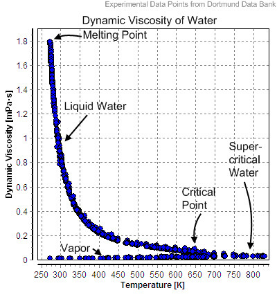