DO/BOD/COD
DO/BOD/COD 용어 설명
1. DO (용존산소)
DO(Dissolved Oxygen)은 수중에 용해되어 있는 산소 즉 용존산소를 말하며,
DO값은 수온이나 기압, 용질에 따라 영향을 받으며 수온의 상승시 감소하고
대기중의 산소분압에 비례하여 증가한다. 또한 수온의 급격한 상승이나
조류의 번식이 심한 경우에 과포화 될 수도 있으나 순수한 물일 경우 20℃,
1기압에서 포화용존산소량은 약 9ppm정도가 된다.
하천 상류의 경우 거의 포화에 가까운 DO량을 보이고 있으나 하류의 경우
하수나 공장폐수 등의 오염으로 인한 유기 부패성 물질 및 기타 환원물질에
의한 소비로 낮게 나타난다. 따라서 DO는 유기물질의 오염정도를 지시
한다고 할 수 있다.
심하게 오염된 물은 용존산소가 부족하여 혐기성 분해가 일어나 부패하게
되고 DO가 2ppm이상이면 악취의 발생은 없으며 4ppm이상이면 청정이 유지
되고 보통 물고기의 생존이 가능하다.
2. BOD (생물화학적 산소요구량)
BOD(Biochemical Oxygen Demand)는 생물화학적 산소요구량으로 어떠한
유기물이 미생물에 의하여 호기성 상태에서 분해하여 안정화시키는데
요구되는 산소량을 말하며 보통 ppm단위로 표시하고 BOD가 높으면
유기물의 오염도가 높음을 의미한다.
물속에서 부착성 미생물에 의해 유기물질이 호기성 분해가 되면 물속에
있는 DO가 소모된다. 만일 산소를 소모하는 속도가 물 속으로 녹아
들어가는 속도보다 빠르면 물은 혐기성 상태가 된다. 혐기성 상태에서는
물고기의 개체수가 감소하고 부패하여 휘발성 물질이 생성된다. 유기물질의
분해속도와 산소의 소모속도는 BOD를 측정함으로 타나낼 수 있다.
일반적으로 폐수내에 존재하는 유기물의 종류는 대단히 많고 각 유기물의
농도를 일일이 구하는 것이 대단히 어려워 폐수내의 유기물질의 종류를
분석하지 않고 호기성 미생물로 합성 또는 산화시키는 데 필요한 산소량을
측정하므로 유기물의 양을 간접적으로 측정할 수 있다. 유기물질이 유입되면
물 속에 서식하는 미생물은 DO를 소모하므로 유입된 유기물의 양이나
종류를 측정하는 것보다 DO를 소비하는 양을 측정하는 것이 훨씬 용이하다.
BOD는 20℃에서 5일간 배양했을 때 배양기간 동안 소모된 산소의 양을
측정하며 그 값을 통상 BOD 또는 BOD5라고 한다. BOD측정 결과를 보면
유기물이 미생물에 의해서 분해 섭취되므로 산소소비량은 시간에 따라
증가하며 7~10일 후에는 탄소화합물에 의한 NOD이외에 질소화합물의 산화
즉, 질산화가 발생하는데 이를 질소 BOD 또는 NOD(Nitrogenous Oxygen Demand)
라고 부르며, BOD5 시험에서 BOD병 내에 질산화를 일으키는 미생물이
존재하면 탄소화합물에 의한 BOD보다 높게 나타나고 도시하수의 경우에는
질산화가 잘 일어나지 않으나 처리된 폐수에서는 질산화가 일어나는
경우가 있다.
3. COD (화학적 산소 요구량)
COD(Chemical Oxygen Demand)는 화학적 산소요구량으로 물속의 피산화성
물질을 산화제인 중크롬산칼륨(K2Cr2O7), 또는 과망간산칼륨(KMnO4)을
이용하여 화학적으로 산화시킬 때 소비되는 산소량을 보통 ppm단위로
표시한다.
COD는 BOD와 더불어 폐수의 유기물 함유도를 간접적으로 나타내는 중요한
지표로 COD는 유기물을 화학적으로 산화시킬 때 얼마만큼의 산소가
화학적으로 소모되는가를 측정한다. 공정시험법에 의하면 산화제를 일정
과잉량을 가하여 일정시간 동안 방치하여 두었다가 소비된 산화제의
양을 산소로 환산하여 COD를 측정한다. COD는 유기물질의 추정을 목적
으로 하는 경우가 많으나 측정치에는 아질산염, 제일 철염, 유화물
등의 무기물과 환원성 물질이 포함되는 반면 안정된 유기물은 측정치에
포함되지 않는다.
일반적인 방법으로 유기물 및 무기물의 전부를 완전 산화시키는 것은
쉬운 일이 아니다. BOD측정은 5일이나 걸리지만 COD는 2시간으로 측정이
가능하여 BOD를 모르는 폐수를 위하여 COD측정이 흔히 채택된다. COD는
화학적으로 산화 가능한 유기물을 산화시키기 위한 산소요구량이지만
BOD는 미생물에 의해서 산화되는 산소요구량이므로 측정치의 차이가
발생되는 경우가 많다. 폐수의 COD가 BOD보다 클 경우에는 폐수내에
생화학적으로 분해가 안되는 물질을 함유하고 있거나 미생물에 독성을
끼치는 물질을 함유하고 있다는 것을 의미하며, 만일 BOD가 COD보다
클 경우에는 BOD측정 중에 질산화가 발생하였거나 또는 COD측정에
방해되는 물질이 폐수 내에 함유되어 있음을 의미한다. 산화제 중
중크롬산칼륨(K2Cr2O7)은 유기물의 약 80%정도를 분해하고 과망간산
칼륨(KMnO4)은 약 60%를 분해하여 COD를 표시한다.
일반적으로 하천이나 도시하천은 BOD값이 사용되며, 공장폐수나 해수등의
오염지표로는 COD값이 많이 사용된다.
Pasted from <http://chemeng.co.kr/site/bbs/board.php?bo_table=xstudy5&wr_id=14&page=&page=>
'상태와 변화' 카테고리의 다른 글
| Mpemba Effect (0) | 2016.09.02 |
|---|---|
| Water의 종류 (0) | 2016.09.02 |
| Vapor_Liquid equilibrium (0) | 2016.09.02 |
| 해수면상에서 표준 대기의 기본 특성치 (0) | 2016.09.02 |
| 물의 경수와 연수 (0) | 2016.09.02 |
Vapor_Liquid equilibrium
Vapor-liquid equilibrium
From Wikipedia, the free encyclopedia
Jump to: navigation, search
Vapor-liquid equilibrium, abbreviated as VLE by some, is a condition where a liquid and its vapor (gas phase) are in equilibrium with each other, a condition or state where the rate of evaporation (liquid changing to vapor) equals the rate of condensation (vapor changing to liquid) on a molecular level such that there is no net (overall) vapor-liquid interconversion. Although in theory equilibrium takes forever to reach, such an equilibrium is practically reached in a relatively closed location if a liquid and its vapor are allowed to stand in contact with each other long enough with no interference or only gradual interference from the outside.
Contents
[hide]
- 1 VLE data introduction
- 4 Vapor-Liquid Equilibrium diagrams
- 5 Raoult's Law
- 6 See also
- 7 External links
- 8 References
[edit] VLE data introduction
The concentration of a vapor in contact with its liquid, especially at equilibrium, is often given in terms of vapor pressure, which could be a partial pressure (part of the total gas pressure) if any other gas(es) are present with the vapor. The equilibrium vapor pressure of a liquid is usually very dependent on temperature. At vapor-liquid equilibrium, a liquid with individual components (compounds) in certain concentrations will have an equilibrium vapor in which the concentrations or partial pressures of the vapor components will have certain set values depending on all of the liquid component concentrations and the temperature. This fact is true in reverse also; if a vapor with components at certain concentrations or partial pressures is in vapor-liquid equilibrium with its liquid, then the component concentrations in the liquid will be set dependent on the vapor concentrations, again also depending on the temperature. The equilibrium concentration of each component in the liquid phase is often different from its concentration (or vapor pressure) in the vapor phase, but there is a correlation. Such VLE concentration data is often known or can be determined experimentally for vapor-liquid mixtures with various components. In certain cases such VLE data can be determined or approximated with the help of certain theories such as Raoult's Law, Dalton's Law, and/or Henry's Law.
Such VLE information is useful in designing columns for distillation, especially fractional distillation, which is a particular specialty of chemical engineers.[1][2][3] Distillation is a process used to separate or partially separate components in a mixture by boiling (vaporization) followed by condensation. Distillation takes advantage of differences in concentrations of components in the liquid and vapor phases.
In mixtures containing two or more components where their concentrations are compared in the vapor and liquid phases, concentrations of each component are often expressed as mole fractions. A mole fraction is number of moles of a given component in an amount of mixture in a phase (either vapor or liquid phase) divided by the total number of moles of all components in that amount of mixture in that phase.
Binary mixtures are those having two components. Three-component mixtures could be called ternary mixtures. There can be VLE data for mixtures with even more components, but such data becomes copious and is often hard to show graphically. VLE data is often shown at a certain overall pressure, such as 1 atm or whatever pressure a process of interest is conducted at. When at a certain temperature, the total of partial pressures of all the components becomes equal to the overall pressure of the system such that vapors generated from the liquid displace any air or other gas which maintained the overall pressure, the mixture is said to boil and the corresponding temperature is the boiling point (This assumes excess pressure is relieved by letting out gases to maintain a desired total pressure). A boiling point at an overall pressure of 1 atm is called the normal boiling point.
[edit] Thermodynamic description of vapor-liquid equilibrium
The field of thermodynamics describes when vapor-liquid equilibrium is possible, and its properties. Much of the analysis depends on whether the vapor and liquid consist of a single component, or if they are mixtures.
[edit] Pure (single-component) systems
If the liquid and vapor are pure, in that they consist of only one molecular component and no impurities, then the equilibrium state between the two phases is described by the following equations:

;

; and

where

and

are the pressures within the liquid and vapor,

and

are the temperatures within the liquid and vapor, and

and

are the molar Gibbs free energies (units of energy per amount of substance) within the liquid and vapor, respectively.[4] In other words, the temperature, pressure and molar Gibbs free energy are the same between the two phases when they are at equilibrium.
An equivalent, more common way to express the vapor-liquid equilibrium condition in a pure system is by using the concept of fugacity. Under this view, equilibrium is described by the following equation:

where

and

are the fugacities of the liquid and vapor, respectively, at the system temperature

and pressure

.[5] Using fugacity is often more convenient for calculation, given that the fugacity of the liquid is, to a good approximation, pressure-independent,[6] and it is often convenient to use the quantity

, the dimensionless fugacity coefficient, which is 1 for an ideal gas.
[edit] Multicomponent systems
This section requires expansion. |

In a multicomponent system, where the vapor and liquid consist of more than one type of molecule, describing the equilibrium state is more complicated. For all components

in the system, the equilibrium state between the two phases is described by the following equations:

;

; and

where

and

are the temperature and pressure for each phase, and

and

are the partial molar Gibbs free energy also called chemical potential (units of energy per amount of substance) within the liquid and vapor, respectively, for each phase. The partial molar Gibbs free energy is defined by:

where

is the (extensive) Gibbs free energy, and

is the amount of substance of component

.
[edit] Boiling point diagrams
Binary mixture VLE data at a certain overall pressure, such as 1 atm, showing mole fraction vapor and liquid concentrations when boiling at various temperatures can be shown as a two-dimensional graph called a boiling point diagram. The mole fraction of component 1 in the mixture can be represented by the symbol x1. The mole fraction of component 2, represented by x2, is related to x1 in a binary mixture as follows:
x1 + x2 = 1
In multi-component mixtures in general with n components, this becomes:
x1 + x2 + ... + xn = 1

Boiling Point Diagram
The preceding equations are typically applied for each phase (liquid or vapor) individually. In a binary boiling point diagram, temperature (T) is graphed vs. x1. At any given temperature where there is boiling going on, vapor with a certain mole fraction is in equilibrium with liquid with a certain mole fraction, often differing from the vapor. These vapor and liquid mole fractions are both on a horizontal isotherm (constant T) line. When an entire range of boiling temperatures vs. vapor and liquid mole fractions is graphed, two (usually curved) lines are made. The lower one, representing boiling liquid mole fraction at various temperatures, is called a bubble point curve. The upper one, representing vapor mole fraction at corresponding temperatures, is called a dew point curve. [1]
These two lines (or curves) meet where the mixture becomes purely one component, where x1 = 0 (and x2 = 1, pure component 2) or x1 = 1 (and x2 = 0, pure component 1). The temperatures at those two points correspond to the boiling points of the two pure components. In certain combinations of components, the two curves may also meet at a point somewhere in between x1 = 0 and x1 = 1. That point represents an azeotrope in that particular combination of components. That point has an azeotrope temperature and an azeotropic composition often represented as a mole fraction. There can be maximum-boiling azeotropes, where the azeotrope temperature is at a maximum in the boiling curves, or minimum-boiling azeotropes, where the azeotrope temperature is at a minimum in the boiling curves.
If one wants to represent a VLE data for a three-component mixture as a boiling point "diagram", a three-dimensional graph can be used. Two of the dimensions would be used to represent the composition mole fractions, and the third dimension would be the temperature. Using two dimensions, the composition can be represented as an equilateral triangle in which each corner representing one of the pure components. The edges of the triangle represent a mixture of the two components at each end of the edge. Any point inside the triangle represent the composition of a mixture of all three components. The mole fraction of each component would correspond to where a point lies along a line starting at that component's corner and perpendicular to the opposite edge. The bubble point and dew point data would become curved surfaces inside a triangular prism, which connect the three boiling points on the vertical temperature "axes". Each face of this triangular prism would represent a two-dimensional boiling point diagram for the corresponding binary mixture. Due to their three-dimensional complexity, such boiling point diagrams are rarely seen. Alternatively, the three-dimensional curved surfaces can be represented on a two-dimensional graph by the use of curved isotherm lines at graduated intervals, similar to iso-altitude lines on a map. Two sets of such isotherm lines are needed on such a two-dimensional graph: one set for the bubble point surface and another set for the dew point surface.
[edit] K values and relative volatility values
There can be VLE data for mixtures of four or more components, but such a boiling point diagram is hard to show in either tabular or graphical form. For such multi-component mixtures, as well as binary mixtures, the vapor-liquid equilibrium data are represented in terms of K values (vapor-liquid distribution ratios)[1][2] defined by
Ki = yi / xi
which are correlated empirically or theoretically in terms of temperature, pressure and phase compositions in the form of equations, tables or graph such as the well-known DePriester charts.[7][8]
For binary mixtures, the ratio of the K values for the two components is called the relative volatility denoted by α

which is a measure of the relative ease or difficulty of separating the two components. Large-scale industrial distillation is rarely undertaken if the relative volatility is less than 1.05 with the volatile component being i and the less volatile component being j.[2]
K values are widely used in the design calculations of continuous distillation columns for distilling multicomponent mixtures.
[edit] Vapor-Liquid Equilibrium diagrams

Vapor-Liquid Equilibrium Diagram
For each component in a binary mixture, one could make a vapor-liquid equilibrium diagram. Such a diagram would graph liquid mole fraction on a horizontal axis and vapor mole fraction on a vertical axis. In such VLE diagrams, liquid mole fractions for components 1 and 2 can be represented as x1 and x2 respectively, and vapor mole fractions of the corresponding components are commonly represented as y1 and y2. [2] Similarly for binary mixtures in these VLE diagrams:
x1 + x2 = 1 and y1 + y2 = 1
Such VLE diagrams are square with a diagonal line running from the (x1=0, y1=0) corner to the (x1=1, y1=1) corner for reference.
These types of VLE diagrams are used in the McCabe-Thiele method to determine the number of equilibrium stages (or theoretical plates; same thing) needed to distill a given composition binary feed mixture into one distillate fraction and one bottoms fraction. Corrections can also be made to take into account the incomplete efficiency of each tray in a distillation column when compared to a theoretical plate.
[edit] Raoult's Law
At boiling and higher temperatures the sum of the individual component partial pressures becomes equal to the overall pressure, which can symbolized as Ptot.
Under such conditions, Dalton's Law would be in effect as follows:
Ptot = P1 + P2 + ...
Then for each component in the vapor phase:
y1 = P1/Ptot, y2 = P2/Ptot, ... etc.
where P1 = partial pressure of component 1, P2 = partial pressure of component 2, etc.
Raoult's Law is approximately valid for mixtures of components between which there is very little interaction other than the effect of dilution by the other components. Examples of such mixtures includes mixtures of alkanes, which are non-polar, relatively inert compounds in many ways, so there is little attraction or repulsion between the molecules. Raoult's Law states that for components 1, 2, etc. in a mixture:
P1 = x1 P01, P2 = x2 P02, etc.
where P01, P02, etc. are the vapor pressures of components 1, 2, etc. when they are pure, and x1, x2, etc. are mole fractions of the corresponding component in the liquid.
Recall from the first section that vapor pressures of liquids are very dependent on temperature. Thus the P0pure vapor pressures for each component are a function of temperature ( T ): For example, commonly for a pure liquid component, the Clausius-Clapeyron equation (not shown here) may be used to approximate how the vapor pressure varies as a function of temperature. This makes each of the partial pressures dependent on temperature also regardless of whether Raoult's Law applies or not. When Raoult's Law is valid these expressions become:
P1(T) = x1 P01(T), P2(T) = x2 P02(T), etc.
At boiling temperatures if Raoult's Law applies, the total pressure becomes:
Ptot = x1 P01(T) + x2 P02(T) + ...
At a given Ptot such as 1 atm and a given liquid composition, T can be solved for to give the liquid mixture's boiling point or bubble point, although the solution for T may not be mathematically analytical (may require a numerical solution or approximation). For a binary mixture at a given Ptot, bubble point T can become a function of x1 (or x2) and this function can be shown on a two-dimensional graph like a binary boiling point diagram.
At boiling temperatures if Raoult's Law applies, a number of the preceding equations in this section can be combined to give the following expressions for vapor mole fractions as a function of liquid mole fractions and temperature:
y1 = x1 P01(T)/Ptot,
y2 = x2 P02(T)/Ptot, ... etc.
Once the bubble point T's as a function of liquid composition in terms of mole fractions have been determined, these values can be plugged into the above equations to obtain corresponding vapor composition in terms of mole fractions. When this is finished over a complete range of liquid mole fractions and their corresponding temperatures, one effectively obtains a temperature ( T ) function of vapor composition mole fractions. This function effectively acts as the dew point T function of vapor composition.
In the case of a binary mixture: x2 = 1 - x1 and the above equations can be expressed as:
y1 = x1 P01(T)/Ptot and
y2 = (1 - x1) P02(T)/Ptot
For many kinds of mixtures, particularly where there is interaction between components beyond simply the effects of dilution, Raoult's Law does not work well for determining the shapes of the curves in the boiling point or VLE diagrams. Even in such mixtures, there are usually still differences in the vapor and liquid equilibrium concentrations at most points, and distillation is often still useful for separating components at least partially. For such mixtures, empirical data is typically used in determining such boiling point and VLE diagrams. Chemical engineers have done a significant amount of research trying to develop equations for correlating and/or predicting VLE data for various kinds of mixtures which do not obey Raoult's Law well.
원본 위치 <http://en.wikipedia.org/wiki/Vapor-liquid_equilibrium>
'상태와 변화' 카테고리의 다른 글
| Water의 종류 (0) | 2016.09.02 |
|---|---|
| DO/BOD/COD (0) | 2016.09.02 |
| 해수면상에서 표준 대기의 기본 특성치 (0) | 2016.09.02 |
| 물의 경수와 연수 (0) | 2016.09.02 |
| MEK (1) | 2016.07.15 |
해수면상에서 표준 대기의 기본 특성치
해수면상의 표준대기의 기본특성치
Temperature : 288.16 K
Pressure : 1.01325x10⁵ N/m2
Density : 1.225 kg/m3
Gas Constant : 287.04 J/kg-K
Specific Heat Ratio : 1.40
Acoustic Speed : 340.29 m/s
Viscosity : 1.7894x10⁻⁵ kg/m-s
Kinematic Viscosity : 1.4607x10⁻⁵ m2/s
Molecular Weight : 28.9644
Pasted from <http://chemeng.co.kr/site/bbs/board.php?bo_table=xstudy5&wr_id=9&page=&page=>
'상태와 변화' 카테고리의 다른 글
| DO/BOD/COD (0) | 2016.09.02 |
|---|---|
| Vapor_Liquid equilibrium (0) | 2016.09.02 |
| 물의 경수와 연수 (0) | 2016.09.02 |
| MEK (1) | 2016.07.15 |
| Unit conversion (0) | 2016.07.13 |
1. 경수/연수
1) 경수 : 경수는 석회염, 칼슘, 마그네슘, 철, 구리, 질산염, 염화염, 실리콘,
나트륨 등의 물질들이 포함되어 있는데 그 중에서도 칼슘과 마그네슘이
가장 많이 용해되어 있다. 이들은 독립된 원소로 용해되어 있는 것이
아니라 중탄산염, 황산염, 질산염 그리고 염화물로 녹아 있습니다.
이처럼 광물질을 함유하고 있는 물을 경수라고 합 니다.
2) 연수 : 연수는 경수에 함유되어 있는 광물질의 양이 낮은 물로서 일반적으로
저수지, 호수, 강에서 취수하는 물을 말합니다.
2. 경도
물의 세기를 나타내는 용어로서 물속에 용존하고 있는 금속 2가
(Ca++, Mg++, Fe++, Mn++, Sr++등) 양이온 농도(㎎/ℓ) 값을
이에 대응하는 탄산칼슘(CaCO3) 으로 환원하여 ㎎/ℓ (ppm)으로
나타낸 것을 말합니다.
1) 종류 : 총경도, 칼슘경도, 마그네슘경도, 미탄산염경도(영구경도),
탄산염경도(일 시경도) 5종이 있습니다.
- 총 경 도 : 수중의 칼슘이온 및 마그네슘이온에 의한 경도
- 칼 슘 경 도 : 수중의 칼슘이온에 의한 경도
- 마그네슘경도 : 수중의 마그네슘에 의한 경도
- 미탄산염경도 : 황산염, 철산염, 황화물 등과 같이 끓임에 따라
석출하지 않는 칼슘 염 및 마그네슘염에 의한 경도(영구 경도)
- 탄산염 경도 : 칼슘과 마그네슘이 수중에 탄산수소염 모양으로 포함되어
있어 끓이면 탄산을 방출하여 탄산칼슘 및 탄산마그네슘이
일시적으로 석출되었다가 다시 가수분해하여 Mg(OH)2가
석출되므로 일시 경도라고도 부름
2) 경수의 영향
가) 가 정
① 세탁 시 비누 사용량의 증가
② 흰색 세탁물의 변색화
③ 의류의 수명 감소
④ 의류에 비누때 및 세제 침적물이 응결
⑤ 보일러 및 배관에 스케일 형성으로 열 효율 감소 및 수명 단축
⑥ 채소, 과일 등의 세척 후 맛의 텁텁함
⑦ 커피나 녹차 등에서 막을 형성하여 맛을 감소시킴
⑧ 각종 무기성 미네랄(칼슘, 마그네슘, 철, 구리 등)은 체내에서
소화/ 흡수가 되지 않아 인체에 축적되어 신장결석, 관절염,
변비 등을 일으키는 원인이됨
나) 산업분야
① 도금공업 : 도금층의 밀착 불량, 피막의 변색, 줄무늬와 반점의 발생
② 섬유염색공업 : 정련 및 세정 불량, 염색의 방해, 방사공정이나
세정공정에서 노즐의 막힘 현상발생
③ 완(반)제품 세척 시 : 얼룩이나 줄무늬가 생김
④ 기타 : 가열기, 배관, 열 교환기, 냉각시스템 등에 스케일이 형성되어
열효율이 감소 및 수명의 단축
3) 경도에 따른 물의 구분
① 연수 (Soft) : 0 ~ 75 mg/ℓ
② 적당한경수 (Moderately Hard) : 76 ~ 150 mg/ℓ
③ 경수 (Hard) : 151 ~300 mg/ℓ
④ 고경수 (Very Hard) : 301 mg/ℓ 이상
[출처 : 웅진코웨이]
Pasted from <http://chemeng.co.kr/site/bbs/board.php?bo_table=xstudy5&wr_id=10&page=&page=>
'상태와 변화' 카테고리의 다른 글
| Vapor_Liquid equilibrium (0) | 2016.09.02 |
|---|---|
| 해수면상에서 표준 대기의 기본 특성치 (0) | 2016.09.02 |
| MEK (1) | 2016.07.15 |
| Unit conversion (0) | 2016.07.13 |
| 용해도 (0) | 2016.07.13 |

Enable interactivity
Interactivity requires the installation of the CDF player.
Share Enlarge Data Customize A Plaintext Interactive Disable Interactivity Download as CDF
Chemical names and formulas:
-
More
Enable interactivity
Interactivity requires the installation of the CDF player.
Share Enlarge Data Customize A Plaintext Interactive Sources
Disable Interactivity Download as CDF
Structure diagram:
- Skeletal structure
- Skeletal structure
- All atoms
- Lewis structure
- Show bond information
-
Step‐by‐step
Enable interactivity
Interactivity requires the installation of the CDF player.
Share Enlarge Data Customize A Plaintext Interactive Sources
Disable Interactivity Download as CDF
3D structure:
-
Show space filling
Enable interactivity
Interactivity requires the installation of the CDF player.
Share Enlarge Data Customize A Plaintext Interactive Disable Interactivity Download as CDF
Basic properties:
-
More
Enable interactivity
Interactivity requires the installation of the CDF player.
-
Units »
Share Enlarge Data Customize A Plaintext Interactive Sources
Disable Interactivity Download as CDF
Liquid properties (at STP):
Enable interactivity
Interactivity requires the installation of the CDF player.
Definitions »
-
Units »
Share Enlarge Data Customize A Plaintext Interactive Sources
Disable Interactivity Download as CDF
Thermodynamic properties:
-
More
Enable interactivity
Interactivity requires the installation of the CDF player.
-
Units »
Share Enlarge Data Customize A Plaintext Interactive Sources
Disable Interactivity Download as CDF
Chemical identifiers:
-
More
Enable interactivity
Interactivity requires the installation of the CDF player.
Share Enlarge Data Customize A Plaintext Interactive Sources
Disable Interactivity Download as CDF
NFPA label:
-
Table
Enable interactivity
Interactivity requires the installation of the CDF player.
Share Enlarge Data Customize A Plaintext Interactive Disable Interactivity Download as CDF
Safety properties:
-
More
Enable interactivity
Interactivity requires the installation of the CDF player.
Share Enlarge Data Customize A Plaintext Interactive Disable Interactivity Download as CDF
Toxicity properties:
-
More


'상태와 변화' 카테고리의 다른 글
| 해수면상에서 표준 대기의 기본 특성치 (0) | 2016.09.02 |
|---|---|
| 물의 경수와 연수 (0) | 2016.09.02 |
| Unit conversion (0) | 2016.07.13 |
| 용해도 (0) | 2016.07.13 |
| 온도변화에 대한 유체의 점도 (0) | 2016.07.09 |
Unit conversion
Unit Conversions
|
PRESSURE CONVERSION TABLE |
|
|
|
|
|
|
|
|
mH2O |
psi |
inHg |
mmHg |
mbar |
Pa |
|
mH2O |
1 |
1.42233 |
2.8959 |
73.55592 |
98.0665 |
9806.65 |
|
psi |
0.70307 |
1 |
2.03602 |
51.71493 |
68.9476 |
6894.757 |
|
inHg |
0.34532 |
0.49115 |
1 |
25.4 |
33.8639 |
3386.388 |
|
mmHg |
0.01359 |
0.01934 |
0.03937 |
1 |
1.3332 |
133.322 |
|
mbar |
0.01019 |
0.0145 |
0.02953 |
0.75006 |
1 |
100 |
|
Pa |
0.000102 |
0.00015 |
0.000295 |
0.0075 |
0.01 |
1 |
|
VELOCITY CONVERSION TABLE |
|
|
|
|
|
|
|
|
cm/s |
ft/s |
m/s |
km/hr |
knots |
mph |
|
cm/s |
1 |
30.48 |
100 |
27.78 |
51.48 |
44.7 |
|
ft/s |
0.03281 |
1 |
3.281 |
0.9113 |
1.689 |
1.467 |
|
m/s |
0.01 |
0.3048 |
1 |
0.2778 |
0.5148 |
0.477 |
|
km/hr |
0.036 |
1.097 |
3.6 |
1 |
1.853 |
1.609 |
|
knots |
0.01943 |
0.5921 |
1.943 |
0.5396 |
1 |
0.8684 |
|
mph |
0.02237 |
0.6818 |
2.237 |
0.6214 |
1.152 |
1 |
|
TEMPERATURE CONVERSION TABLE |
|
|
|
CONVERT FROM |
CONVERT TO |
FORMULA |
|
Fahrenheit |
Celsius |
(F - 32) / 1.8 |
|
Fahrenheit |
Kelvin |
(F + 459.67) / 1.8 |
|
Fahrenheit |
Rankine |
F + 459.67 |
|
Rankine |
Kelvin |
R / 1.8 |
|
Rankine |
Celsius |
(R - 491.67) / 1.8 |
|
Rankine |
Fahrenheit |
R - 459.67 |
|
Celsius |
Fahrenheit |
(1.8 x C) + 32 |
|
Celsius |
Rankine |
(1.8 x C) + 491.67 |
|
Celsius |
Kelvin |
C + 273.15 |
|
Kelvin |
Rankine |
1.8 x K |
|
Kelvin |
Fahrenheit |
(1.8 x K) - 459.67 |
|
Kelvin |
Celsius |
K - 273.15 |
|
DENSITY CONVERSION TABLE |
|
|
|
|
|
kg/m3 |
slugs/ft3 |
lbm/ft3 |
|
kg/m3 |
1 |
0.00194 |
0.0624 |
|
slugs/ft3 |
515.3788 |
1 |
32.17096 |
|
lbm/ft3 |
16.02 |
0.03108 |
1 |
Pasted from <http://www.flowkinetics.com/conversions.htm>
'상태와 변화' 카테고리의 다른 글
| 물의 경수와 연수 (0) | 2016.09.02 |
|---|---|
| MEK (1) | 2016.07.15 |
| 용해도 (0) | 2016.07.13 |
| 온도변화에 대한 유체의 점도 (0) | 2016.07.09 |
| Empirical formula Water, steam, gas (0) | 2016.07.09 |
용해도(1)
1. 용해와 용액
(1) 용해 : 한 물질이 다른 물질에 녹아 고르게 섞여 들어가는 현상
(2) 용액 : 두 가지 이상의 서로 다른 물질이 고르게(균일하게) 섞여 있는 혼합물
① 용매 : 물, 알코올, 벤젠 등 다른 물질을 녹이는 물질
② 용질 : 소금, 설탕 등과 같이 용매에 녹아 들어가는 물질
③ 액체와 액체의 혼합물의 경우 양이 많은 물질을 용매, 양이 적은 물질을 용질로 구분
한다.
(3) 용해의 원리: 용매 분자와 용질 분자 사이의 인력이 용질 분자 간이나 용매 분자 간의
인력보다 크면 용해가 잘 일어난다.
(4) 용액의 성질
① 어느 부분이나 성질이 같은 균일 혼합물이다.
② 대체로 투명한 액체이며, 용질 입자가 보이지 않는다.
③ 오래 두어도 침전물이 생기지 않으며 거름종이에 걸러도 걸러지는 것이 없다.
(5) 고체 물질의 용해 속도
① 용질 입자를 작게 만들수록 용해 속도가 빠르다.
② 흔들거나 유리 막대로 저어 주면 용해 속도가 빠르다.
③ 온도가 높을수록 용해 속도가 빠르다.
(6) 용액의 종류 : 용매에 따라 구분한다.
① 용매가 물인 경우 : 수용액
② 용매가 알코올인 경우 : 알코올 용액
2. 용해될 때의 부피와 질량의 변화
(1) 질량의 변화: 용해가 일어날 때 용매와 용질의 알갱이의 수에는 변화가 없으므로 녹기
전후의 질량에는 변화가 없다.
ㆍ용액의 질량 = 용매의 질량 + 용질의 질량
(2) 부피의 변화 : 용해가 일어나면 그 부피는 각각의 부피를 합한 것보다 감소한다. 이것은
서로 섞이는 용매와 용질의 알갱이의 크기가 달라서 큰 알갱이들 사이로 작은 알갱이들이
끼어 들어가기 때문이다.
ㆍ용액의 부피 < 용매의 부피 + 용질의 부피
3. 농도
(1) 용액의 농도 : 용액의 진한 정도
① 용액의 농도는 용질의 질량과 용매의 질량에 따라 달라진다.
② 용액의 농도에 따라 색, 맛, 밀도, 끓는점, 어는점 등이 달라진다.
(2) 퍼센트 농도 : 용액 100g 속에 녹아 있는 용질의 양을 g수로 나타낸 것
|
ㆍ퍼센트 농도(%) = |
용질의 질량 |
× 100 |
|
|
용액의 질량 |
|

용해도(2)
1. 포화와 포화 용액
(1) 포화 : 일정한 온도에서 일정량의 용매에 용질이 최대로 녹아 있는 상태
① 포화 용액 : 포화 상태에 있는 용액으로 용질을 더 넣어도 용해되지 않고 바닥에 가라
앉는다.
② 불포화 용액 : 용질이 녹을 수 있는 양보다 덜 녹아 있어서 용질을 더 녹일 수 있는 상
태의 용액을 말한다.
③ 과포화 용액 : 용액을 천천히 냉각시키면 냉각된 용액에서 녹을 수 있는 양보다 많은
양의 고체가 녹아 있게 되는데 이러한 용액을 과포화 용액이라고 한다.
2. 용해도와 용해도 곡선
(1) 용해도 : 일정한 온도에서 용매 100g에 녹는 용질의 최대 g수를 그 온도에서의 용해도
라고 한다.
① 온도와 용해도 : 일반적으로 고체 용질의 용해도는 온도가 높을수록 커진다.
|
온도 (℃) |
황산구리 |
소금 |
염화칼슘 |
백반 |
붕산 |
|
20 |
26 |
35 |
43 |
11 |
4 |
|
50 |
34 |
37 |
55 |
36 |
11 |
|
80 |
55 |
38 |
59 |
54 |
23 |
[표] 고체 물질의 용해도
② 용매와 용해도 : 물질의 용해도는 용매의 종류에 따라 다르다.
③ 용해도의 표시 : 용해도를 나타낼 때는 용질의 종류와 용매의 종류 및 온도를 함께 표
시해야 한다.
④ 일정 온도, 일정 용매에서의 용해도는 물질마다 다르므로 물질을 구별하는 특성이
된다.
(2) 용해도 곡선 : 온도에 따른 물질의 용해도를 그래프로 나타낸 것
① 용해도 곡선으로 각 물질의 용해도를 비교해 볼 수 있다.

② 용액의 % 농도를 구할 수 있다.
③ 용액이 냉각될 때 석출되는 용질의 g수를 계산해 낼 수 있다.
ㆍ석출되는 용질의 양
= 처음에 녹아 있던 용질의 양 - 냉각시킨 온도에서 녹을 수 있는 양

용해도(3)
1. 고체 및 액체의 용해도
(1) 고체 및 액체의 용해도 : 대체로 온도가 높을수록 증가하며, 압력의 영향은 거의 받지
않는다.
① 온도와 고체의 용해도 : 일반적으로 용매에 고체가 용해되려면 고체 표면으로부터
입자들이 떨어져 나와야 하므로, 즉 고체 분자의 운동이 활발해지므로 열에너지가
필요하다. 따라서 대부분 고체 물질의 용해 과정에서는 열을 흡수하게 되고 열을 가
해 줄수록 용해도가 증가한다.
② 용해 과정이 열을 방출하는 경우에는 온도가 낮을수록 용해도가 증가하는데, 이런 경
우는 드물다.
예) 황산세륨
③ 고체 분자는 액체 분자에 비하여 분자 운동이 느리므로 액체 분자와 잘 섞이기 위해
서는 고체 분자의 운동이 더 활발해져야 한다. → 온도를 높이면 고체 분자의 운동이
활발해져 액체에 잘 녹는다.

2. 기체의 용해도
(1) 기체의 용해도는 온도가 낮을수록, 압력이 높을수록 커진다. 기체의 용해도는 온도와 압
력에 따라 크게 변하므로 기체의 용해도를 나타낼 때 온도와 압력을 함께 나타내야 한다.
(2) 기체의 용해도와 온도 : 액체에 녹는 기체 분자는 기체 상태에서보다 운동 에너지가 낮은
상태에 있다. 온도가 높아지면 용액 속의 기체 분자의 운동이 활발해져 용액 밖으로 튀어
나오기 때문에 용해도는 감소한다.
→ 온도가 낮으면 기체 분자의 운동이 감소되어 액체 분자의 운동과 비슷해지므로 잘 섞
인다.

(3) 기체의 용해도와 압력 : 기체의 압력이 커지면 기체의 부피가 줄어들고 밀도는 증가한다.
따라서, 액체 표면에 충돌하는 기체의 분자수가 증가하여 더 많은 수의 기체 분자가 용
액에 녹아 들어가게 되므로 용해도가 증가하게 된다.
'상태와 변화' 카테고리의 다른 글
| MEK (1) | 2016.07.15 |
|---|---|
| Unit conversion (0) | 2016.07.13 |
| 온도변화에 대한 유체의 점도 (0) | 2016.07.09 |
| Empirical formula Water, steam, gas (0) | 2016.07.09 |
| 기체운동이론 (0) | 2016.07.09 |
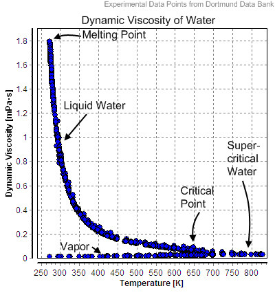
온도변화에 대한 유체의 점도

원본 위치 <http://upload.wikimedia.org/wikipedia/commons/6/6a/Dynamic_Viscosity_of_Water.png>
온도 변화에 대한 물의 점도 변화
|
- t - (oF) |
- μ - (lb s/ft2) x 10-7 |
- ν - (ft2/s) x 10-4 |
|
-40 |
3.29 |
1.12 |
|
-20 |
3.34 |
1.19 |
|
0 |
3.38 |
1.26 |
|
10 |
3.44 |
1.31 |
|
20 |
3.50 |
1.36 |
|
30 |
3.58 |
1.42 |
|
40 |
3.60 |
1.46 |
|
50 |
3.68 |
1.52 |
|
60 |
3.75 |
1.58 |
|
70 |
3.82 |
1.64 |
|
80 |
3.86 |
1.69 |
|
90 |
3.90 |
1.74 |
|
100 |
3.94 |
1.79 |
|
120 |
4.02 |
1.89 |
|
140 |
4.13 |
2.01 |
|
160 |
4.22 |
2.12 |
|
180 |
4.34 |
2.25 |
|
200 |
4.49 |
2.4 |
|
300 |
4.97 |
3.06 |
|
400 |
5.24 |
3.65 |
|
500 |
5.8 |
4.51 |
|
750 |
6.81 |
6.68 |
|
1000 |
7.85 |
9.30 |
|
1500 |
9.50 |
15.1 |
Absolute and Kinematic Viscosity of Air at Standard Atmospheric Pressure - SI Units:

|
- t - (K) |
- μ - (kg/m s) x 10-5 |
- ν - (m2/s) x 10-6 |
|
100 |
0.6924 |
1.923 |
|
150 |
1.0283 |
4.343 |
|
200 |
1.3289 |
7.490 |
|
250 |
1.488 |
9.49 |
|
300 |
1.983 |
15.68 |
|
350 |
2.075 |
20.76 |
|
400 |
2.286 |
25.90 |
|
450 |
2.484 |
28.86 |
|
500 |
2.671 |
37.90 |
|
550 |
2.848 |
44.34 |
|
600 |
3.018 |
51.34 |
|
650 |
3.177 |
58.51 |
|
700 |
3.332 |
66.25 |
|
752 |
3.481 |
73.91 |
|
800 |
3.625 |
82.29 |
|
850 |
3.765 |
90.75 |
|
900 |
3.899 |
99.30 |
|
950 |
4.023 |
108.2 |
|
1000 |
4.152 |
117.8 |
|
1100 |
4.44 |
138.6 |
|
1200 |
4.69 |
159.1 |
|
1300 |
4.93 |
182.1 |
|
1400 |
5.17 |
205.5 |
|
1500 |
5.40 |
229.1 |
|
1600 |
5.63 |
254.5 |
- 1 N s/m2 = 1 Pa s = 10 poise = 1,000 milliPa s
- 1 m2/s = 1 x 104 cm2/s =1 x 10⁴ stokes = 1 x 10⁶ centistokes
- Kinematic viscosity converter
-
|
Density of air 1) (lb/ft3) |
|
|
|
|
|
|
|
|
|
|
|
|
|
Air temperature (oF) |
Gauge Pressure (psi) |
|
|
|
|
|
|
|
|
|
|
|
|
|
0 |
5 |
10 |
20 |
30 |
40 |
50 |
60 |
70 |
80 |
90 |
100 |
|
30 |
0.081 |
0.109 |
0.136 |
0.192 |
0.247 |
0.302 |
0.357 |
0.412 |
0.467 |
0.522 |
0.578 |
0.633 |
|
40 |
0.080 |
0.107 |
0.134 |
0.188 |
0.242 |
0.295 |
0.350 |
0.404 |
0.458 |
0.512 |
0.566 |
0.620 |
|
50 |
0.078 |
0.105 |
0.131 |
0.185 |
0.238 |
0.291 |
0.344 |
0.397 |
0.451 |
0.504 |
0.557 |
0.610 |
|
60 |
0.076 |
0.102 |
0.128 |
0.180 |
0.232 |
0.284 |
0.336 |
0.388 |
0.440 |
0.492 |
0.544 |
0.596 |
|
70 |
0.075 |
0.101 |
0.126 |
0.177 |
0.228 |
0.279 |
0.330 |
0.381 |
0.432 |
0.483 |
0.534 |
0.585 |
|
80 |
0.074 |
0.099 |
0.124 |
0.174 |
0.224 |
0.274 |
0.324 |
0.374 |
0.424 |
0.474 |
0.524 |
0.574 |
|
90 |
0.072 |
0.097 |
0.121 |
0.171 |
0.220 |
0.269 |
0.318 |
0.367 |
0.416 |
0.465 |
0.515 |
0.564 |
|
100 |
0.071 |
0.095 |
0.119 |
0.168 |
0.216 |
0.264 |
0.312 |
0.361 |
0.409 |
0.457 |
0.505 |
0.554 |
|
120 |
0.069 |
0.092 |
0.115 |
0.162 |
0.208 |
0.255 |
0.302 |
0.348 |
0.395 |
0.441 |
0.488 |
0.535 |
|
140 |
0.066 |
0.089 |
0.111 |
0.156 |
0.201 |
0.246 |
0.291 |
0.337 |
0.382 |
0.427 |
0.472 |
0.517 |
|
150 |
0.065 |
0.087 |
0.109 |
0.154 |
0.198 |
0.242 |
0.287 |
0.331 |
0.375 |
0.420 |
0.464 |
0.508 |
|
200 |
0.060 |
0.081 |
0.101 |
0.142 |
0.183 |
0.244 |
0.265 |
0.306 |
0.347 |
0.388 |
0.429 |
0.470 |
|
250 |
0.056 |
0.075 |
0.094 |
0.132 |
0.170 |
0.208 |
0.246 |
0.284 |
0.322 |
0.361 |
0.399 |
0.437 |
|
300 |
0.052 |
0.070 |
0.088 |
0.123 |
0.159 |
0.195 |
0.230 |
0.266 |
0.301 |
0.337 |
0.372 |
0.408 |
|
400 |
0.046 |
0.062 |
0.078 |
0.109 |
0.141 |
0.172 |
0.203 |
0.235 |
0.266 |
0.298 |
0.329 |
0.360 |
|
500 |
0.041 |
0.056 |
0.070 |
0.098 |
0.126 |
0.154 |
0.182 |
0.210 |
0.238 |
0.267 |
0.295 |
0.323 |
|
600 |
0.038 |
0.050 |
0.063 |
0.089 |
0.114 |
0.140 |
0.165 |
0.190 |
0.216 |
0.241 |
0.267 |
0.292 |
|
Density of air 1) (lb/ft3) |
|
|
|
|
|
|
|
|
|
|
|
|
|
Air temperature (oF) |
Gauge Pressure (psi) |
|
|
|
|
|
|
|
|
|
|
|
|
|
120 |
140 |
150 |
200 |
250 |
300 |
400 |
500 |
700 |
800 |
900 |
1000 |
|
30 |
0.743 |
0.853 |
0.909 |
1.185 |
1.460 |
1.736 |
2.29 |
1.84 |
3.94 |
4.49 |
5.05 |
5.60 |
|
40 |
0.728 |
0.836 |
0.890 |
1.161 |
1.431 |
1.702 |
2.24 |
2.78 |
3.86 |
4.40 |
4.95 |
5.49 |
|
50 |
0.717 |
0.823 |
0.876 |
1.142 |
1.408 |
1.674 |
2.21 |
2.74 |
3.80 |
4.33 |
4.87 |
5.40 |
|
60 |
0.700 |
0.804 |
0.856 |
1.116 |
1.376 |
1.636 |
2.16 |
2.68 |
3.72 |
4.24 |
4.76 |
5.28 |
|
70 |
0.687 |
0.789 |
0.840 |
1.095 |
1.350 |
1.605 |
2.12 |
2.63 |
3.65 |
4.16 |
4.67 |
5.18 |
|
80 |
0.674 |
0.774 |
0.824 |
1.075 |
1.325 |
1.575 |
2.08 |
2.58 |
3.58 |
4.08 |
4.58 |
5.08 |
|
90 |
0.662 |
0.760 |
0.809 |
1.055 |
1.301 |
1.547 |
2.04 |
2.53 |
3.51 |
4.00 |
4.50 |
4.99 |
|
100 |
0.650 |
0.747 |
0.795 |
1.036 |
1.278 |
1.519 |
2.00 |
2.48 |
3.45 |
3.93 |
4.42 |
4.90 |
|
120 |
0.628 |
0.721 |
0.768 |
1.001 |
1.234 |
1.467 |
1.933 |
2.40 |
3.33 |
3.80 |
4.26 |
4.73 |
|
140 |
0.607 |
0.697 |
0.742 |
0.967 |
1.193 |
1.418 |
1.868 |
2.32 |
3.22 |
3.67 |
4.12 |
4.57 |
|
150 |
0.597 |
0.686 |
0.730 |
0.951 |
1.173 |
1.395 |
1.838 |
2.28 |
3.17 |
3.61 |
4.05 |
4.50 |
|
200 |
0.552 |
0.634 |
0.675 |
0.879 |
1.084 |
1.289 |
1.698 |
2.11 |
2.93 |
3.34 |
3.75 |
4.16 |
|
250 |
0.513 |
0.589 |
0.627 |
0.817 |
1.088 |
1.198 |
1.579 |
1.959 |
2.72 |
3.10 |
3.48 |
3.86 |
|
300 |
0.479 |
0.550 |
0.586 |
0.764 |
0.941 |
1.119 |
1.475 |
1.830 |
2.54 |
2.90 |
3.25 |
3.61 |
|
400 |
0.423 |
0.486 |
0.518 |
0.675 |
0.832 |
0.989 |
1.303 |
1.618 |
2.25 |
2.56 |
2.87 |
3.19 |
|
500 |
0.379 |
0.436 |
0.464 |
0.604 |
0.745 |
0.886 |
1.167 |
1.449 |
2.01 |
2.29 |
2.58 |
2.86 |
|
600 |
0.343 |
0.394 |
0.420 |
0.547 |
0.675 |
0.802 |
1.057 |
1.312 |
1.822 |
2.08 |
2.33 |
2.59 |
1) Density is based on atmospheric pressure 14.696 psia and molecular weight of air 28.97
- density - 1 lb/ft3 = 16.018 kg/m3
- pressure - 1 psi (lb/in2) = 6,894.8 Pa (N/m2)
- temperature - T(oC) = 5/9[T(oF) - 32]
-
Density of air can also be expressed as
ρ = 1.325 pin Hg / TR (1)
where
ρ = density (lb/ft3)
pin Hg = pressure (inches Hg)
TR = absolute temperature (Rankine)
원본 위치 <http://www.engineeringtoolbox.com/air-temperature-pressure-density-d_771.html>
원본 위치 <http://www.engineeringtoolbox.com/air-absolute-kinematic-viscosity-d_601.html>
Common properties for air are indicated the table below
|
- t - (oC) |
- ρ - (kg/m3) |
Specific heat capacity - cp - (kJ/kg K) |
Thermal conductivity - l - (W/m K) |
- ν - (m2/s) x 10-6 |
Expansion coefficient - b - (1/K) x 10-3 |
Prandtl's number - Pr - |
|
-150 |
2.793 |
1.026 |
0.0116 |
3.08 |
8.21 |
0.76 |
|
-100 |
1.980 |
1.009 |
0.0160 |
5.95 |
5.82 |
0.74 |
|
-50 |
1.534 |
1.005 |
0.0204 |
9.55 |
4.51 |
0.725 |
|
0 |
1.293 |
1.005 |
0.0243 |
13.30 |
3.67 |
0.715 |
|
20 |
1.205 |
1.005 |
0.0257 |
15.11 |
3.43 |
0.713 |
|
40 |
1.127 |
1.005 |
0.0271 |
16.97 |
3.20 |
0.711 |
|
60 |
1.067 |
1.009 |
0.0285 |
18.90 |
3.00 |
0.709 |
|
80 |
1.000 |
1.009 |
0.0299 |
20.94 |
2.83 |
0.708 |
|
100 |
0.946 |
1.009 |
0.0314 |
23.06 |
2.68 |
0.703 |
|
120 |
0.898 |
1.013 |
0.0328 |
25.23 |
2.55 |
0.70 |
|
140 |
0.854 |
1.013 |
0.0343 |
27.55 |
2.43 |
0.695 |
|
160 |
0.815 |
1.017 |
0.0358 |
29.85 |
2.32 |
0.69 |
|
180 |
0.779 |
1.022 |
0.0372 |
32.29 |
2.21 |
0.69 |
|
200 |
0.746 |
1.026 |
0.0386 |
34.63 |
2.11 |
0.685 |
|
250 |
0.675 |
1.034 |
0.0421 |
41.17 |
1.91 |
0.68 |
|
300 |
0.616 |
1.047 |
0.0454 |
47.85 |
1.75 |
0.68 |
|
350 |
0.566 |
1.055 |
0.0485 |
55.05 |
1.61 |
0.68 |
|
400 |
0.524 |
1.068 |
0.0515 |
62.53 |
1.49 |
0.68 |
원본 위치 <http://www.engineeringtoolbox.com/air-properties-d_156.html>


'상태와 변화' 카테고리의 다른 글
| Unit conversion (0) | 2016.07.13 |
|---|---|
| 용해도 (0) | 2016.07.13 |
| Empirical formula Water, steam, gas (0) | 2016.07.09 |
| 기체운동이론 (0) | 2016.07.09 |
| 온도 (0) | 2016.07.09 |
Empirical formula Water, steam, gas
==============================================================
Empirical Formula of thr flow of Water, Steam, Gas
==============================================================
◎ Hazen and Williams Equation (Only water flow)
Q = 0.000599 d^2.63 c ((p1 - p2)/L)^0.54
Q : flow rate [l/min]
d : internal diameter [mm]
c : constant
140 - new steel pipe
130 - new cast iron pipe
110 - riveted pipe
p1 : inlet pressure [bar_g]
p2 : outlet pressure [bar_g]
L : length [m]
◎ Babcock Equation (Only steam flow)
△p = 6.76 ((d + 91.45)/d^6) W^2 L V
△p : pressure [bar_g]
d : internal diameter [mm]
W : flow rate [kg/hr]
L : length [m]
V : specific volume [m3/kg]
◎ Spitzglass 식 (Low pressure gas; 7kPa 이하)
q = 0.00338 √((△hw d^5)/(Sg L (1+ 91.5/d + 0.00118*d)))
q : flow rate [m3/hr] (@ 15℃, 1.013 bar_a)
hw : static pressure head [mm H2O]
d : internal diameter [mm]
Sg : specific gravity of gas [ ]
L : length [m]
◎ Weymouth 식 (High pressure gas)
q = 0.00261 d^2.667 √[((p1^2-p2^2) / (Sg Lm)) * (288/T)]
q : flow rate [m3/hr] (@ 15℃, 1.013 bar_a)
d : internal diameter [mm]
p1 : inlet pressure [bar_a]
p2 : outlet pressure [bar_a]
Sg : specific gravity of gas [ ]
Lm : length [km]
T : absolute temperature [K]
[이 게시물은 운영자님에 의해 2008-03-22 00:48:37 유체역학에서 이동 됨
원본 위치 <http://www.chemeng.co.kr/site/bbs/board.php?bo_table=xstudy2&wr_id=61&page=3>


풍선을 불면 커지는 이유는 풍선 내부의 기체가 풍선의 안쪽에 힘을 가하기 때문이다. <출처: gettyimage>
공기가 들어있는 풍선이나 타이어는 외부에서 힘(압력)이 작용해도 어느 한도 내에서는 그 형태를 그대로 유지한다. 내부에 들어있는 기체들이 벽면에 힘(압력)을 가하기 때문이다. 기체는 어떻게 공간을 차지하고 압력을 미치는가?
고체나 액체와 구별되는 기체의 특징은 구성분자(원자)들 간의 평균거리이다. 액체나 고체 상태의 분자들은 이웃 분자들과의 거리가 가까워서 전자기적 힘으로 그 형태를 유지하지만, 기체 상태의 분자들은 이웃 분자들과의 거리가 상당히 멀어서 상호작용이 미약할 뿐 아니라 분자들 자체의 부피도 아주 작아서 기체가 차지하는 공간은 대부분 텅 비어 있다고 볼 수 있다. 그런데 기체는 어떻게 외부 압력에 대해서 부피를 유지할까? 결론부터 말하면 기체가 용기 벽에 가하는 압력은 분자들이 벽에 충돌하면서 가하는 힘에 기인한다. 그리고 기체 분자들의 수가 매우 많아서 수없이 많은 충돌의 충격이 연속적인 힘을 가하는 것처럼 느껴지는 것이다.
기체의 성질을 설명하는 기체운동이론

이상기체모형을 설명한 그림. <출처: (cc) A. Greg(Greg_L) at Wikimedia.org>
기체분자들이 용기 벽에 미치는 압력은 기체모형에 뉴턴의 역학법칙을 적용하여 구할 수 있다. 물리학자들은 눈으로 볼 수 없는 물체나 현상들에 대한 유추로서 모형(model)을 사용하는데 기체에 대한 한 가지 모형은 기체분자를 점 입자로 보고, 입자들 사이에는 완전탄성충돌 외에는 다른 상호작용이 없이 자유롭게 움직인다고 간주하는 것이다.
이러한 기체 모형을 이상기체모형이라고 한다. 이상기체모형에 뉴턴역학과 통계학의 방법을 적용하여 기체의 운동을 미시적으로 다룰 수 있는데 이 분야를 기체운동이론이라고 한다.
기체운동이론을 적용하여 용기내의 기체 압력을 구할 수 있다. 방법은 기체분자 하나가 벽면에 미치는 압력을 뉴턴의 역학법칙을 이용하여 구한 다음, 용기(부피: V) 내의 모든 기체분자들(분자수: N)에 대한 평균량으로 기체의 압력(P)을 구하는 것이며 결과는 다음과 같다.

여기서 우리가 알 수 있는 것은 기체의 압력은 기체의 밀도(개수밀도: N/V)와 평균운동에너지(<k>)에 비례한다는 것이다. 실제 기체들 중에서 여기에 해당하는 기체들은 원자 하나가 분자를 이루는 불활성기체(He, Ne 등)들이다.
온도는 분자들의 평균운동에너지의 척도
화학자들은 밀도가 낮은 기체들의 경우 압력(P)과 부피(V), 그리고 온도(T) 사이에는 다음과 같은 간단한 관계가 성립함을 실험적으로 알아냈다.

이 양은 기체의 분자수(N)에 비례하므로 비례상수(k: 볼츠만상수)를 도입하여 다음과 같이 쓸 수 있다.

따라서 위의 두 식으로부터 기체의 평균운동에너지는 다음과 같음을 알 수 있다.

이 식은 기체분자들의 운동에너지가 온도에 비례함을 말해준다. 이것은 다시 말해 온도라는 물리량이 기체들의 평균운동에너지를 나타내는 척도임을 말해주는 것이다.

부풀린 풍선을 액체 질소로 냉각시키면 부피가 줄어든다. <출처: 저자 제공>

기구에 열을 가하면 크게 부풀어 오른다. <출처: Gettyimage>
기체분자들은 어떻게 공간을 가득 채우는가?
기체 분자는 질량이 매우 작아서 주위로부터 아주 작은 에너지만 얻어도 빠르게 운동하기 시작한다. 예를 들어 상온(20℃)에서 산소분자의 평균운동에너지는 아래와 같이 매우 작다.

이 때문에 기체분자들은 아주 쉽게 상온에서 에너지(열)를 얻어서 운동을 시작한다. 그리고 기체분자들은 매우 빠르게 움직이면서 공간을 가득 채우게 된다.
기체분자들은 얼마나 빠르게 움직이고 있나?
기체 분자들의 평균운동에너지로부터 기체분자들의 평균운동속도를 다음과 같이 구할 수 있다.

상온에서 기체분자들은 상당히 빠른 속도로 움직이고 있다. 예를 들어 상온의 대기압에서 산소분자들의 평균속도는 vrms=480m/s정도이다. 그런데 이 속도는 대기 중의 음파의 속도와 비슷한데, 음파는 공기분자들 사이의 충돌에 의해서 전달되는 것이다. 그런데 냄새가 퍼지는 속도는 이렇게 빠르지 않다. 그 이유는 무엇일까? 대기 중의 기체 분자 수가 매우 많아서 기체분자들 사이에 수많은 충돌이 일어나기 때문이다. 그러면 기체분자가 충돌을 일으킨 후 다음 충돌을 일으킬 때까지 얼마나 이동할까? 이 거리(평균자유행로: Λ, 람다)는 분자의 지름(d)과 밀도(N/V)에 따라 다음과 같이 결정된다.

예를 들어 공기 중의 질소분자(d=0.3nm)는 상온에서 0.1 μm(100nm) 정도이다. 이 거리는 이웃 기체 분자들 간의 평균거리(약 4nm)의 약 25배에 해당한다.
기체분자들은 얼마나 자주 충돌하나?
상온에서 공기 중의 질소분자(속력: 약 500m/s)는 다른 분자들과 초당 약 50억 회의 충돌을 일으킨다. 분자들의 충돌을 눈으로 알아보기 어렵지만 한 가지 확실한 증거는 브라운운동이다. 영국의 식물학자 로버트 브라운(1879-1955)은 현미경을 통하여 물에 떠 있는 꽃가루 입자가 매우 불규칙하게 움직이는 것을 발견하였는데 공기 중의 연기입자의 운동에서도 관찰된다.

공기 중 연기입자는 브라운 운동을 한다.

평면상의 브라운 운동을 컴퓨터 프로그램으로 제작한 그림.
브라운운동이 유체분자와 부유입자의 충돌로 설명할 수 있음을 증명한 사람은 바로 아인슈타인이다. 부유입자는 유체분자들의 충돌로 인해 유체분자와 동일한 평균운동에너지를 갖지만 질량이 훨씬 크기 때문에 현미경으로 볼 수 있을 정도의 속도로 움직이는 것이 브라운 운동임이 밝혀졌다.
글
김충섭 | 수원대학교 물리학과 교수
서울대학교 물리학과를 졸업하고 동 대학에서 박사학위를 받았다. 현재 수원대학교 물리학과 교수이다. 저서로 [동영상으로 보는 우주의 발견], [메톤이 들려주는 달력 이야기], [캘빈이 들려주는 온도 이야기] 등이 있다.
발행2012.01.02.
출처: <http://navercast.naver.com/contents.nhn?rid=20&contents_id=7196>
'상태와 변화' 카테고리의 다른 글
| 온도변화에 대한 유체의 점도 (0) | 2016.07.09 |
|---|---|
| Empirical formula Water, steam, gas (0) | 2016.07.09 |
| 온도 (0) | 2016.07.09 |
| 평형 (0) | 2016.07.09 |
| 변화 (0) | 2016.07.09 |
